NLP - Climate Change Misinformation Detection

COMP90042: Natural Language Processing

In this age of Internet, information sharing is at its peak. We can easily read and share content on different platforms without actually verifying the authenticity of the information. Due to this, misinformation and fake content is on the rise, which can be tackled and predicted using machine learning algorithms. In this project, we present a misinformation detection system for climate change related content that can classify text to be either correct information or misleading information. In order to implement such system, we propose different methodologies with their experimental results and error analysis.

Introduction

Climate change is one of the hottest topic of discussion in several conferences and debates. One of the major factor that contributes to this continuing debate is the widespread use of social media and news platforms to deliver and spread misinformation. In order to tackle and handle such problem, we can use natural language processing to build language models that can understand and distinguish between correct and fake content.
In this paper, we propose several methodologies which aims at building a supervised binary classifier model that can classify provided text into negative and positive label, where positive label means text is delivering some kind of misinformation. In order to train such classifier with supervised learning methods, we need training data with both positive and negative labels. The training corpus is provided with only positive labels, so we need to enhance it with negative labels. We achieve this by scraping several authentic website articles which gives correct information about climate change.
This is followed by data preprocessing pipeline which includes several methods to clean and process data which can be later integrated with machine learning models. With this preprocessed data, we explored several feature extraction techniques such as bag of words, frequency transformations with different importance weights as stated by @Leopold2002. We have also explored improved feature space such as Delta-TF-IDF as proposed by @Martineau2009, Word2Vec corpus embeddings and pretrained [@glove] word vectors. These feature extraction techniques are trained on several models and tuned on development data, which is then followed by detailed error analysis of these techniques.
As per our experimental results, word2vec average word embeddings [@Elsaadawy2018] learned on the training corpus with 10 ReLu units deep learning model outperformed other methodologies on the provided test data.

Data Extraction and Analysis

In order to enhance training corpus with negative labels, data needs to be extracted from external sources. We have used the article URLs provided by the @climateurls2020 which is a contextual dataset for exploring climate change narratives with more than 6.3M news articles. We are using dataset curated in 2020 which contains 1.08M article links.
In order to extract the information, this dataset is loaded using pandas and each row is checked for extraction using ’climate-change’ keyword. Then, @newspaper3k python package is used to download and parse articles using URLs. After parsing, text is extracted and saved for each row. This process is then repeated until 1500 articles are extracted. Using this extraction approach, training corpus is enhanced with 1500 negative labels, making it suitable to build a binary classifier.
We then analysed the training data to understand basic pattern or relationship of texts with the problem. Firstly, we analysed the distribution of part-of-speech tags across positive and negative labels as shown in the below figure.

It can be deduced from the plot that content words are dominating the training corpus. Also, there is a substantial score of punctuation and numbers which can be eliminated in preprocessing phase to decrease the feature space. Similarly, we can analyse the word counts for uni-grams across positive and negative labels to understand their distribution.

As per the above plot, most of the misinformation are based on the word related to ’climate’, ’energy’ or ’temperature’. These words are being contradicted by the unigrams in the negative label. This plot gives us an initution that distribution of unigrams is not highly skewed, thereby unigrams can provide good feature space for building models. Moreover, we saw that distribution of bigrams, trigrams and fourgrams is extremely skewed in terms of the word counts which makes them inappropriate for feature representation.

Data Preprocessing

Data cleanup and preprocessing is one of the most important aspect for effective modelling of the problem. As shown in POS figure, there is a very high score of function words which includes stop words, conjunctions and other non-important words. These words can be eliminated along with punctuation and numbers which will eventually decrease the learning feature space. We also performed lemmatization and used NLTK word synsets to further identify the relevant words for our analysis. This data cleanup and transformation pipeline is shown in below figure.

We run this preprocessing pipeline for each text in the training corpus, development corpus and test corpus to either get cleaned text in lemma form or get lemma tokens for each cleaned text. This preprocessed data is then used for feature extraction and feed into machine learning models for label predictions.

Proposed Methodologies

In this section, we propose different approaches to perform feature extraction from the preprocessed training corpus and train machine learning models for getting effective accuracy results on the development and test data.

Approach 4.1: Bag-of-words feature representation

We first started with the bag-of-words feature extraction method to get our baseline model. We used unigrams to create this representation as their distribution across labels is not extremely skewed as compared to bigrams, trigrams and four-grams. In order to build this representation, we used the raw frequencies transformation scheme as described by @Leopold2002 which uses raw counts of words across documents. This creates a bag-of-words matrix which is then trained on several models, tuned on the development data and tested on the test data.

Approach 4.2: TF-IDF feature representation

In this approach, we use the concept of importance weights to increase the weights of the words that are important for classifying labels. We use inverse document frequency (IDF) weight scheme as proposed by @Leopold2002 which calculates the weight for each word $w$ in a text collection consisting of N documents as:

\[idf_w = log\frac{N}{df_w}\]

where, $df_w$ is the number of documents in the collection which contains the word $w$. This yields a weight vector which is multiplied with raw frequencies used in the previous approach to generate TF-IDF matrix. This matrix is then normalized with L2-normalization so as to improve convergence of the machine learning algorithms.

Approach 4.3: TF-Redundancy feature representation

In this approach, we use different importance weighting scheme called redundancy as proposed by @Leopold2002 with the possibility that it might provide better weight adjustments than previous IDF approach. We calculate the redundancy weight for each word $w$ in a text collection of N documents as:

\[r_w = log\:N + \sum_{i=1}^{N}\frac{f(w,d_i)}{f(w)}log\frac{f(w,d_i)}{f(w)}\]

where $f(w,d_i)$ is the frequency of word $w$ in the document $d_i$ and $f(w)$ is the frequency of word in the entire collection of documents. This yields a weight vector which is again multiplied with raw frequencies and scaled to its maximum absolute value (MaxAbsScaler) to generate TF-redundancy matrix. These weights provides a measure of how much is the distribution of the term $w$ deviating from the uniform distribution, thereby quantifying the skewness of a probability distribution.

Approach 4.4: TF-Delta-IDF feature representation

In this approach, we use another weighting scheme called Delta-IDF as proposed by @Martineau2009. In this scheme, the weight of the term $w$ is calculated as:

\[\Delta idf_w = log_2 \left(\frac{N_w}{P_w}\right)\]

where $N_w$ is the number of documents with term $w$ in a negatively labeled training set and $P_w$ is the number of documents with term $w$ in a positively labeled training set. This yields a weight vector which is multiplied with raw frequencies and scaled to its maximum absolute value (MaxAbsScaler) to generate TF-Delta-IDF matrix. The idea of this scheme is to represent true importance of words within the documents that can help the algorithm to classify them more effectively.

Approach 4.5: Average Word2Vec Embeddings

In this approach, we created our own scheme to generate importance weights for the word by averaging word2vec embeddings as proposed by @Elsaadawy2018. We have used Word2Vec training model provided by gensim to learn word vectors of size 100 on the training corpus. We trained our model on unigrams using skip-grams approach with the window size of 2. We have also used negative sampling of size 20 for generating embeddings. These embeddings produced for each word $w$ in the corpus are averaged and used as the weight for the word in the documents to create a weight matrix which is then scaled using MaxAbsScaler. This weight matrix is used as the feature representation to train machine learning models.

Approach 4.6: Pretrained Word2Vec Embeddings

In this approach, we use pretrained model called @glove which contains 6B tokens with 400K vocabulary words. We used this layer as the embedding layer for the deep learning models with GloVe weight vectors of size 300 which are trained while the model is training. This layer is then trained with several deep learning models like CNN and LSTM and tuned on the development data to get the most effective precision and recall for our analysis.

Experimental Results

In this section, we present the results of our proposed methodologies on the precision, recall and F1-score metric for the positive class. We also show the most optimal model that worked with our methodology and present results on both development and test data.

Method	Model	Precision	Recall	F1-score
Approach 4.1	LSVC(C=3.25)	0.93	0.78	0.85
Approach 4.2	LSVC(C=1.5)	0.93	0.74	0.82
Approach 4.3	LSVC(C=0.015)	0.81	0.84	0.82
Approach 4.4	LSVC(C=0.025)	0.80	0.86	0.83
Approach 4.5	10 ReLU	0.95	0.72	0.82
Approach 4.6	10 LSTM	0.88	0.74	0.80

As per above table, we can see that Approach 4.1 produced best F1-score on the development set, where highest recall can be achieved by Approach 4.4 and best precision by Approach 4.5. Similarly, we can show results of these approaches on the test data as shown by codalab.

Method	Model	Precision	Recall	F1-score
Approach 4.1	LSVC(C=3.25)	0.5062	0.82	0.6260
Approach 4.2	LSVC(C=1.5)	0.5556	0.80	0.6557
Approach 4.3	LSVC(C=0.015)	0.4828	0.84	0.6131
Approach 4.4	LSVC(C=0.025)	0.5000	0.84	0.6269
Approach 4.5	10 ReLU	0.5714	0.88	0.6929
Approach 4.6	10 LSTM	0.5634	0.80	0.6612

Clearly, Approach 4.5 outperforms every other approaches on the results produced on the codalab. This approach is able to generalize extremely well on the unseen data with comparatively better precision and recall. The final score of this approach is shown in the below table.

Method	Model	Precision	Recall	F1-score
Approach 4.5	10 ReLU	0.5743	0.85	0.6855

Error Analysis

In this section, we provide explanation and reasoning why some approaches worked better than the other on the development data and able to generalise well on the test data.

Approach 4.1: The bag-of-words approach with LinearSVC is not able to classify 16 documents correctly from the dev set. The distribution of words for misclassified labels across positive and negative corpus can be shown using below bar chart.

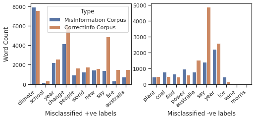
We can clearly see from the left chart that certain words are more prominent in the negative label corpus than positive label corpus due to which these documents are misclassified as correct information. Similarly, we can see the same pattern for ’coal’, ’find’ or ’power’ word in the right chart, where ’say’ seems to be having less impact towards reducing classification error.

Approach 4.2: We can correct above shown problem using weighting scheme like IDF that assigns weights to the word as per their frequency across documents. But, this approach still takes into account the term frequency due to which those 16 documents are still not correctly classified.

Approach 4.3: This approach tries to quantify the skewness of the term to improve the weights but fails to overcome the effect of term frequency and provides almost similar result as of IDF scheme.

Approach 4.4: This approach tries to improve weighting scheme for the word by assigning more negative weights to the word in the positive corpus and more positive weights to the word in the negative corpus which is enhanced by the term frequency. Again, this approach suffers from the ambiguous words problem that are almost equally distributed across both corpus.

Approach 4.5: This approach tries to eliminate term frequency and calculate weights for the word by averaging Word2Vec learned vectors that captures semantic similarity among words. We are able to get best precision using this approach but it fails to provide good recall and f1-score for positive class. One of the reason is the large amount of words are common across positive and negative labels as shown in unigrams figure, due to which word2vec is not able to understand correct context of the word with the window size of 2. Moreover, huge amount of information is lost upon taking mean of the vectors.

Approach 4.6 This approach tries to retain the loss of information by keeping entire 300 length word vector learned for each word by using embedding layer. These word vectors are taken from GloVe pretrained model but they are not able to improve classification results for development set due to inconsistent cosine similarity for the words that are not valid in the provided context and less coverage of around 46% with the vocabulary of the training corpus.

Conclusion

We proposed several methodologies for representing features and used machine learning models to identify climate change misinformation. We compared the results with development and test set where average word2vec embeddings approach with 10 ReLu units and sigmoid layer provides the best precision on the development set and generalizes better on the test set.

Future Work

We can enhance proposed methodologies by exploring contextual representations using BERT or ELMo which might solve context ambiguity problem with better word embeddings. We can also explore topic modelling using LDA that might help us to filter out content not related to climate change. Moreover, transfer learning implementations like ULMFiT can also be explored for this problem.

Cheers!