
Artificial Intelligence - Pacman Capture The Flag
Our task was to develop an autonomous Pacman agent team to play the Pacman Capture the Flag Contest by suitably modifying file myTeam.py (and maybe some other auxiliarly files you may implement). The code submitted should be internally commented at high standards and be error-free and never crash.
We’ll be first explaining all the approaches we have implemented for creating an efficient AI pacman agent in Design Choices section and then critically analyzing these approaches in Experiments and Evaluation section. We have also added the link to our youtube presentation after wiki documentation.
Complete github project: AI-capture-the-flag-pacman-contest
We were able to achieve 43/45 overall project marks:
| Component | Course Weight |
|---|---|
| Performance of the preliminary submission | 9.8/10 |
| Performance of the final submission | 14.5/10 |
| Quality of Wiki and types of techniques used | 10/10 |
| Quality of Video and types of techniques used | 9.1/10 |
| Total | 43.4/45 |
Table of Contents
Design Choices
Approach One: BFS and A* Heuristic Search
Our goal is to find an optimal path from the current location to the goal location. We need to different goal states depending on the current game state. For example, the defensive agent can aim for own food location or enemy Pacman in our boundary, while for offensive agent goal will be enemy food or running back to the entry point.
We have used the breadth-first search as the blind search algorithm and A* as the heuristic search algorithm. Hence, we will be discussing both the methodologies in the given section.
Implementation: myTeamHeuristicAgent.py
BFS and A* Agent Architecture
For both the search algorithms, the underlying architecture is the same. The only difference is in the way heuristic function exploits the power of A* by defining a heuristic function to find the optimal path.
In this section, we are going to explain the architecture of our blind search and heuristic agent. We used different architecture for both offensive and defensive agents.
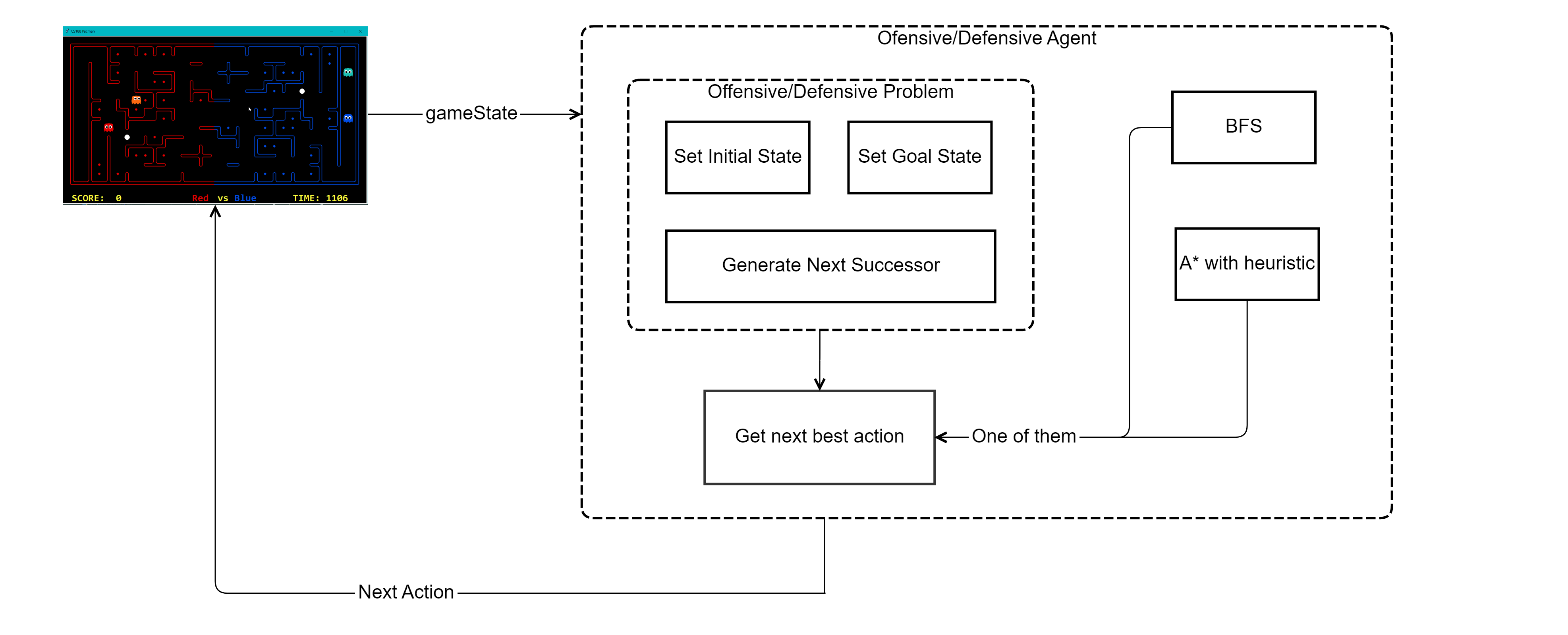
We used the architecture like a decision tree plan in the game to decide the goal states and found the optimal path from the current state to the goal state. Step of action calculation are as follow.
- Step-1 (Executed once): Agent registers the initial state of the game and the starting position. This is same for both the offensive and defensive agents.
- Step-2: Both the agents have methods defined for choosing the action. Here we define the problem. For offensive agent, we have offensiveProblem, and for a defensive agent, we have defined defensiveProblem. These problems are defined such that they can be passed to both BFS and A* for the generating the list of action to reach the goal state.
- Step-3: Agents use the respective problem classes to define the problem and pass this to the search algorithm (BFS or A*) to find the list of actions.
- Step-4: We find the optimal plan for using the search method. Optimal plan is a list of actions, and we select the first action to be the next action for the agent. This action will lead to a new game state, and we need to repeat the above-mentioned steps are to find the next action in the new game state.
Offensive Agent
In this section, we are going to discuss design strategies and decision for the implementation of the offensive agent and offensiveProblem definition.
Offensive Motivation
The objective of this agent is to acquire as much food as possible without being eaten by the enemy and return to our area. The score is increased in our favour only when the agent can safely return to its own territory. If it gets eaten on the enemy territory, it loses all food and returns to its original state. We can also turn on the power mode for our agent by eating the enemy capsule. In this state, we can eat as much food as we wish without worrying about the enemy and can even eat him/her if we cross path. We need to consider these factors while deciding the goal state for the offensiveProblem.
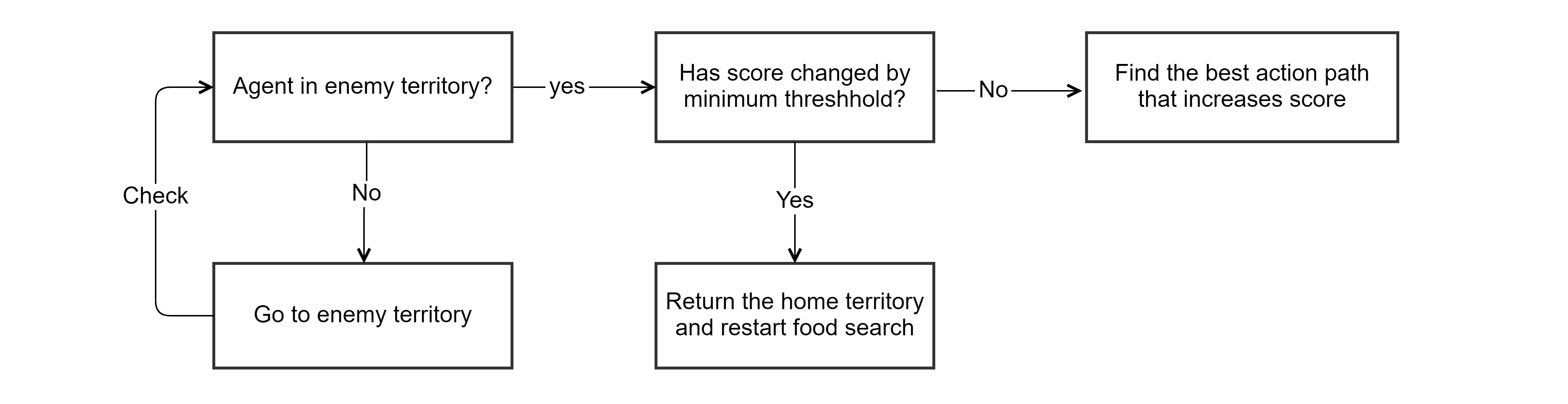
Offensive Governing Strategy
We have used the following logic to decide the action for the offensive agent. The goal state in the problem statement is to increase the game score by a minimum threshold. The search algorithms use generate successor methods of the problem statement that in turn uses the generateSuccessor() function provided by the gameState. This function provides the entire game state, including the situation where the agent dies and reaches the initial game position. Hence we can focus on score improvement, and search algorithm provides us with the path that eats the food, avoids the enemy, east the capsule if required and returns to home territory.
Offensive Problem Implementation
Problem definition for the offensive agent consists of following main methods.
- Initializing the problem
- Setting initial state
- Checking goal state
- Generating the successors
Offensive Heuristic Implementation
The offensive heuristic function is called when using A* search algorithm. It is based on the distance to the closest food until score change occurs, as per the goal state definition. For more details, check function offensiveHeuristic() defined in heuristicTeam.py.
Defensive Agent
In this section, we are going to discuss design strategies and decision for the implementation of the defensive agent and defensiveProblem definition.
Defensive Motivation
The objective of this agent is to protect the food in our territory and chase of the enemy Pacman by eating them. Goal states for defensive agents are vague and require good domain implementation to define good strategy. Our agent can eat enemy Pacman. Except for games states where our agent is in scaring state due to enemy eating our capsule. Our governing strategy needs to implement for this situation. A good strategy will make sure that the enemy is not able to enter the territory, and if they enter, we need to minimize the amount of food they eat or protecting all food by eating the enemy.
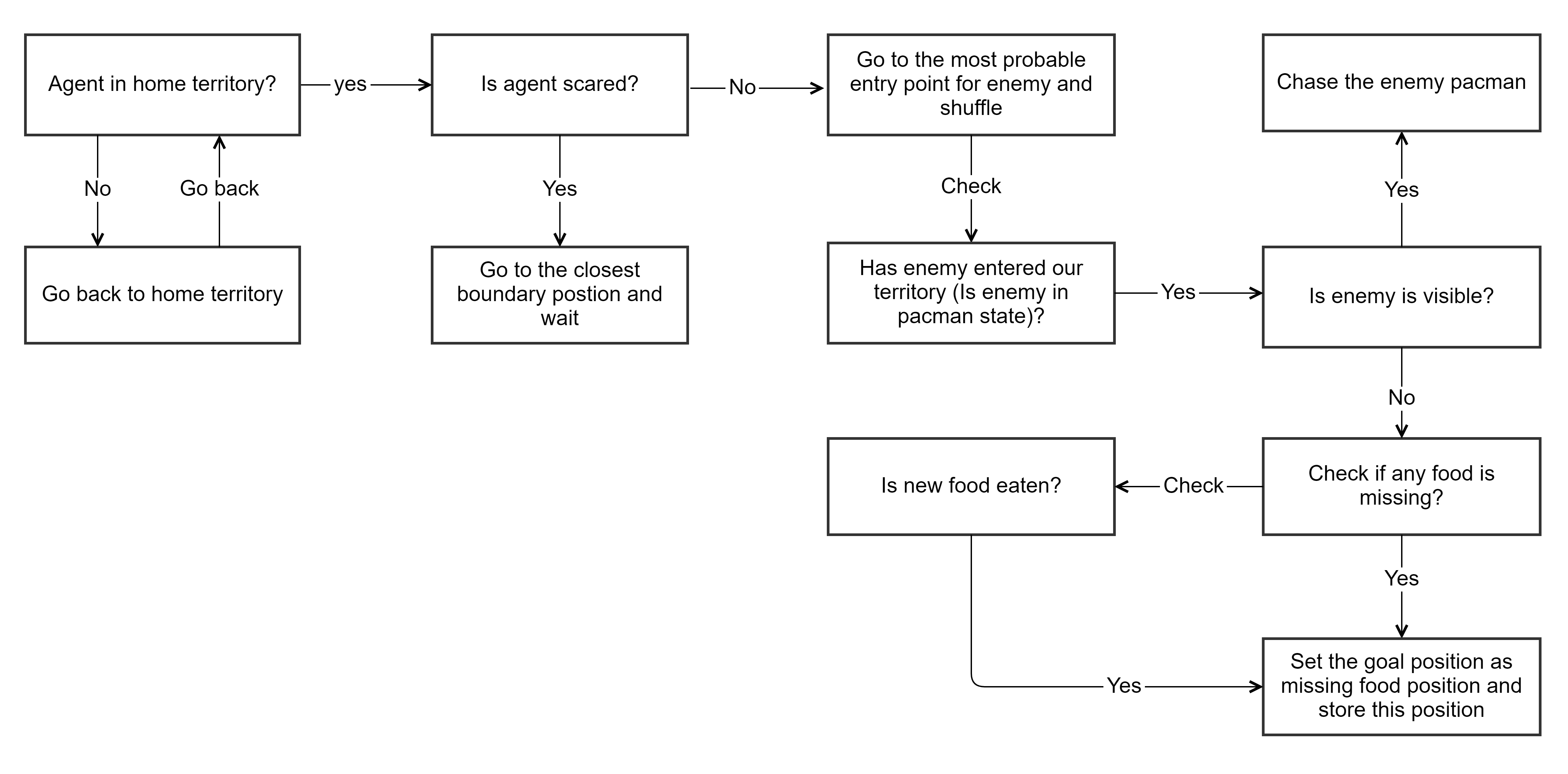
Defensive Governing Strategy
We have used the following logic to decide the action for the defensive agent. We have to reevaluate the goal state after every step since the defensive agent has no clear goal state except for an objective of protecting food and eating the enemy. We also need to have a strategy when enemy Pacman eats the capsule and is in power mode. Our agent waits at the boundary position since once the scared state is over, this will be the best point to stop the enemy. We also have implemented a logic to find the best entry positions for the enemy to enter. If we are already on boundary position, we check for other viable boundary positions where the enemy can enter, based on the distance of these positions to our food. We activate this logic once the enemy is has breached our territory. Once the enemy eats our food that becomes our goal position until we either see the enemy or he/she eats next food. If we see the enemy, then chase holds the highest priority.
Defensive Problem Implementation
Problem definition for the defensive agent consists of following main methods.
- Initializing the problem
- Setting initial state
- Checking goal state
- Generating the successors
Defensive Heuristic Implementation
The defensive heuristic function is called when using A* search algorithm. It uses a heuristic function that finds the shortest path to the goal state in a given problem by keeping the heuristic value as the maze distance from the goal and every other action as infinity. This heuristic is neither consistent nor admissible. However, it finds the shortest path to reach the destination with the least node expansion. Since out of the list of actions returned from search algorithms, we only choose only one action, we don’t face any issue with action but save a lot of computation time. For more details check function defensiveHeuristic() defined in heuristicTeam.py.
Application
We used these agents for a couple of competitions in the initial games and found that it relied heavily on the governing strategies and the heuristic functions. It requires time for tuning to improve. These agents performed decently on the games but were able to beat the staff_team_basic. We also were able to beat the staff_team_medium but not the staff_ staff_team_top or staff_team_super teams except for one game each. We found that in the case where goals are clear blind search can provide good action plans.
Trade-offs
Advantages
- Blind search and A* heuristic search algorithms are easy to implement.
- With a good governing-strategy, both the algorithms can provide a good action plan. BFS can provide with the optimal plan.
Disadvantages
- The goal state definition is dependent on the problem definition, which follows a governing strategy. We need to decide the goal state at each stage explicitly. If the strategy is not optimal, then we the optimal output from the search algorithms will not be useful.
- Blind search algorithm implementations have a huge drawback where it cannot look ahead while planning, which can lead to taking a path that leads to risky paths and corner food. It cannot anticipate future states that well.
- A* provides some advantage over the blind search, but it still depends heavily on the heuristic function. A wrong heuristic can produce suboptimal or no solution.
- Search algorithms are dependent on the size of game states. For huge maps, they can be computationally heavy and might not provide appropriate results in the given time limit.
Future improvements
Way to pass the information from one agent to others. This can help plan an enemy chase or food eating strategy. Agents can change the goal states by shuffling the offensiveProblem and defensiveProblem. This will require some decision trees but can produce better results than the existing solution for this approach.
Approach Two: Classical Planning
In this wiki, we will be explaining the usage of Classical Planning (PDDL) in our project. We will first explain the architecture used for implementing classical planning which is followed by its corresponding domain and problem implementation for both offensive and defensive agents. We will also demonstrate their strategies using decision trees with advantages, disadvantages, and future improvements for the PDDL approach.
Implementation: myTeamPDDLAgent.py
Classical Planning Agent Architecture
In this section, we are going to explain our designed classical planning agent architecture that we have used for both offensive and defensive agents. All of the components of the architecture are shown in the below image.
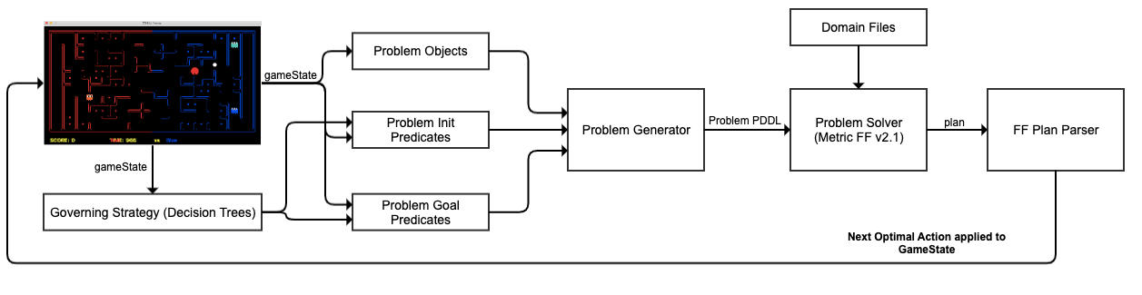
Using this architecture, we can generate a plan for our agent and parse it to get the next most optimal action for execution. The steps of how an action is identified for an agent can be stated as follows.
- Step-1 (Executed once): We first capture the current state of the game and use it to create our problem objects once by registering it in the initial state.
- Step-2: For the consecutive states of the game, we capture the game state and decide different initial and goal predicates for our problem as per the governing strategy. This governing strategy is different for an offensive and defensive agent, as discussed in the strategies section of the agents below.
- Step-3: After the strategy is decided and problem objects, initial predicates, and goal predicates are created, we combine them by using a problem generator to create a problem PDDL file for either offensive or defensive agent.
- Step-4: This problem PDDL file is then provided to our problem-solver, which is using
Metric FF v2.1planner to generate a corresponding plan. We providepacman-domain.pddlfor our offensive agent andghost-domain.pddlfor our defensive agent to get the required plan from the solver. - Step-5: Once the solver generates the plan, we pass it to our FF plan parser engine that in turn derives the next most optimal action that an agent can take.
Finally, we pass the next most optimal action generated by our planner to the gaming engine for execution on our agent. This will lead to a new game state, and the above steps are again repeated for getting the new action.
Offensive Agent
In this section, we are going to explain the strategies and design patterns implemented for creating our offensive classical planning agent.
Motivation
The general idea for creating this agent is to implement aggressive and hostile behavior in our Pacman. Our objective is to make this agent responsible for crossing and entering into the enemy boundary and eat their food by surviving the ghost. To eat food and survive ghost optimally, this agent will use the help of a classical planning solver, which will solve a well-defined problem in a particular situation. In addition to this, the agent will also take the help of different strategies which will help in increasing the chances of survival and coming back home without losing the food.
Pacman Domain Implementation
To use any classical planning solver, we need a well-defined problem domain PDDL file. So, we have created a domain file from the perspective of our offensive agent. The predicates of our implementation can be stated as follows.
- Predicate for whether our offensive agent is at a particular location
locor not. - Predicate for whether given food
food_iis at a particular locationlocor not. - Predicate for whether there is a ghost at a particular location
locor not. - Predicate for whether game state cells are connected or not. This helped us to model walls in the problem file.
- Predicate for whether our offensive agent is carrying food or not.
- Predicate whether the capsule is eaten by our agent or not.
- Predicate whether our agent wants to die or not. This is used for modeling if the agent is being cornered or stuck and can’t get to the capsule, food, or home, then the agent should be able to commit suicide for re-spawning.
- Predicate for whether the agent committed suicide or not.
Similarly, we can represent actions for our offensive agent using the table shown below.
| Action | Precondition | Effect |
|---|---|---|
| move | Allowed if the path is connected and there is no ghost | Agent goes from -> to |
| move-no-restriction | Allowed if path is connected | Agent goes from -> to |
| eat-food | Allowed if the agent is at a food location and food is present | Agent eats the food |
| eat-capsule | Allowed if the agent is at a capsule location and the capsule is present | Agent eats the capsule |
| get-eaten | Allowed if an agent wants to die | Agent commits suicide |
Using this domain file, we can solve the problem statement generated using the game state.
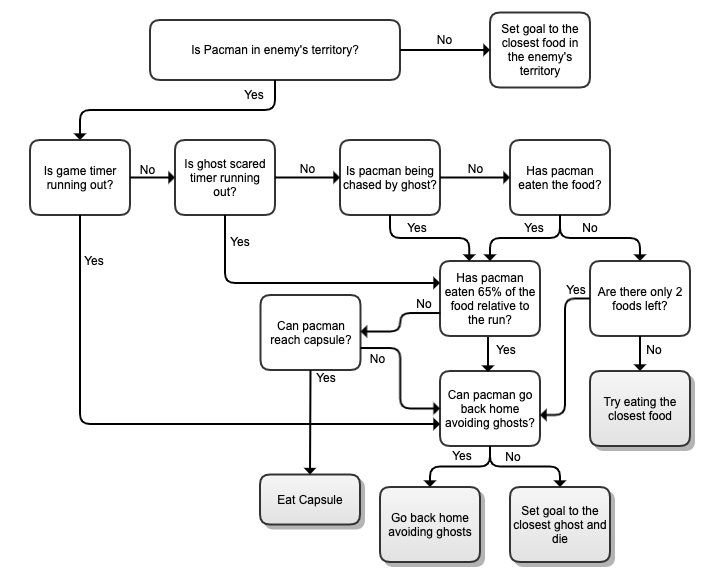
Offensive Governing-Strategy
The governing-strategy for our offensive agent can be described using the below decision tree. The main objective of our offensive agent is to decide whether to eat the capsule, eat the closest food, go back home avoiding ghosts or die if there is no plan found to go back home.
Defensive Agent
In this section, we are going to explain the strategies and design patterns implemented for creating our defensive classical planning agent, which is similar to the Offensive Agent.
Motivation
The general idea for creating this agent is to implement a defensive mindset on our Pacman. Our objective is to make this agent responsible for guarding our food against the enemy Pacman or eat the enemy Pacman when insight. To protect our food and chase the enemy Pacman, this agent will use the help of classical planning solver and domain-specific heuristics which will solve a well-defined problem in a particular situation. In addition to this, the agent will also take the help of different strategies which will help in increasing the chances of guarding our food or trying to eat the enemy Pacman (stopping them from stealing our food).
Ghost Domain Implementation
To use any classical planning solver, we need a well-defined problem domain PDDL file. So, we have created a domain file from the perspective of our defensive agent. The predicates of our implementation can be stated as follows.
- Predicate for whether our defensive agent is at a particular location
locor not. - Predicate for whether there is an enemy at a particular location
locor not. - Predicate for whether game state cells are connected or not. This helped us to model walls in the problem file.
- Predicate for where the location of our capsule we are guarding is.
Similarly, we can represent actions for our offensive agent using the table shown below.
| Action | Precondition | Effect |
|---|---|---|
| move | Allowed if path is connected | Agent goes from -> to |
| kill-invader | Allowed if path is connected and an enemy pacman is in the next cell | Agent goes from -> to and delete invader |
Using this domain file, we can solve the problem statement generated using the game state.
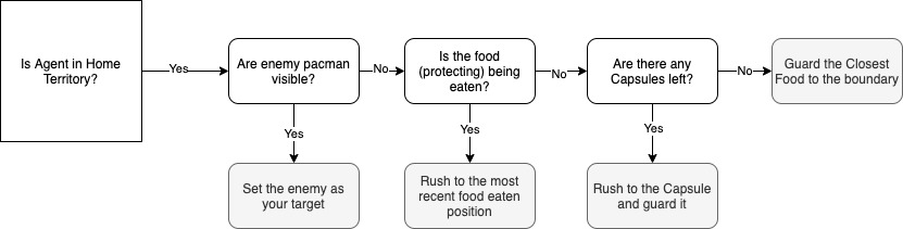
Defensive Governing-Strategy
The governing-strategy for our defensive PDDL agent can be described using the below decision tree.
Trade-offs
Advantages
- Easy to Implement. Once you formulate the game in the Domain (both defensive and offensive) it is easy to generate Problem files during the game dynamically as it requires quick state values for the current stage with respect to the goals. The planner returns a plan calculated best for that situation.
- Does not require explicit coding for setting desired goals as the planner finds the optimal path. For example, for our Pacman to select which food to eat, we formulate all the food as objects in our problem and set
eat-foodto true as our goal (in our predicated explained above). The planner returns the path to the closest food automatically.
Disadvantages
- The planning based implementation has a huge drawback where it cannot look ahead while planning. The disadvantage this brings to the game is it makes our offensive agent (Pacman) really susceptible to being cornered (dead-end), and we cannot anticipate the movement that should be taken in the future.
Future improvements
Classical planning can be improved by adding more predicates that can incorporate future anticipated states of the game. Due to the static nature of the problem statement required by classical planning, the engine can be improved to generate problems that can include complicated objects and fluents which will further improve the search space for the classical planning problem solver.
Approach Three: Model-based MDP (Value Iteration)
In this section, we will be explaining the usage of model-based MDP with value iteration in our project. We attempted the value iteration algorithm on our offensive agent by modeling the game state as the MDP model. The results were not satisfactory so we haven’t pursued this approach in greater depth.
Implementation: myTeamMdpAgent.py
MDP Agent Architecture
In this section, we are going to explain the model-based MDP architecture for our agent. All of the components of the architecture are shown in the below image.
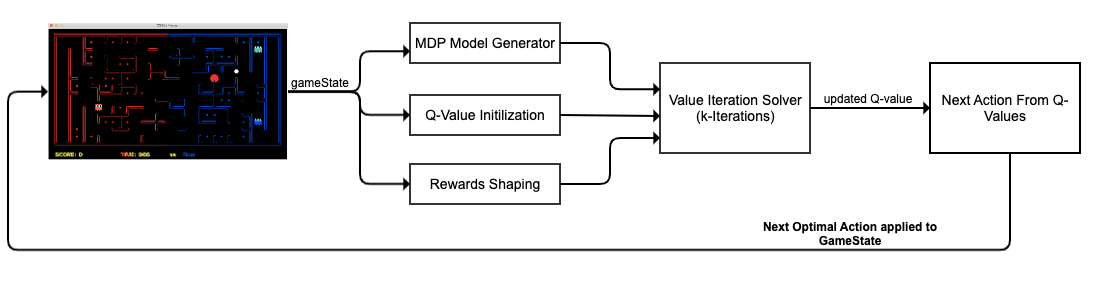
Using this architecture, we are able to generate the next most optimal action for execution. The steps of how an action is identified for an agent can be stated as follows.
- Step-1: We first capture the current game state and use it to create an MDP based model that is required by the value iteration algorithm.
- Step-2: Next, we use the game state to initialize our Q-values with the understanding of terminal states.
- Step-3: Then, we use the current game state to perform the required reward shaping for clearly defining rewards and handling different scenarios.
- Step-4: These components are then provided to the problem solver that is using value iteration to learn Q-values based on the provided rewards. This solver runs for provided
kiterations. - Step-5: After iterations are completed, we take the next best possible action from the updated Q-values.
Finally, we pass the next most optimal action to the gaming engine for execution on our agent. This will lead to a new game state and the above steps are again repeated for getting the new action.
Offensive Agent
In this section, we are going to explain the strategies and design patterns implemented for creating our offensive model-based MDP agent.
Motivation
The general idea for creating this agent is to implement aggressive and hostile behavior in our Pacman. Our objective is to make this agent responsible for crossing and entering into the enemy boundary and eat their food by surviving the ghost. In order to eat food and survive ghost optimally, this agent will use the help of reward shaping to put accurate rewards on the ghosts and the foods. Then, using the value iteration algorithm, the agent will try to learn a policy by which food can be eaten without going through the ghost.
Implementation
As discussed in the architecture above, we first converted our current game state into a valid MDP model. In order to do this, we used the following MDP model structure so that it can be adapted to other MDP solvers.
class gameStateMdpModel(MDP):
    '''
      MDP Model for GameState
    '''
    def __init__(self, gameState, index): ...

    def getStates(self, agentX): ...

    def getStartState(self): ...

    def getPossibleActions(self, state): ...

    def getTransitionStatesAndProbs(self, state, action): ...

    def getReward(self, state, action, nextState): ...

    def isTerminal(self, state): ...
For Q-value initialization, we identified the provided food locations and visible ghost locations as the terminal states.
For rewards shaping, we used the following initial rewards for the foods and the ghosts as shown below.
  self.foodReward = 1.0
  self.ghostReward = -3.0
Food rewards are then manipulated according to the game state and conditions as shown below.
...
features['ghostDistance'] = 1/ghostDistance
self.values[foodPos] = self.mdp.foodReward * features * weights
...
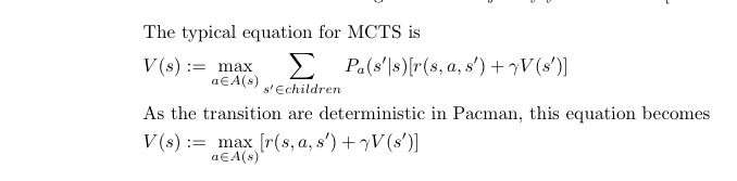
Finally, we can pass all the above components into our value iteration solver which is going to compute Q-values for different states using the below equation.
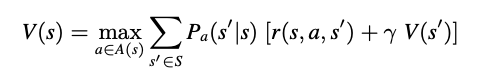
In our game state MDP model, we considered the transition probabilities as 1 since there is no uncertainty with the movement of Pacman agent. This equation is then implemented using the below code, which is used to update Q-values at every iteration.
nextActionWithProbs = self.mdp.getTransitionStatesAndProbs(state, action)
for nextState, prob in nextActionWithProbs:
    qValue += prob * (self.mdp.getReward(state, action, nextState) +
                      self.discount * self.getValueOfState(nextState))
Governing-Strategy
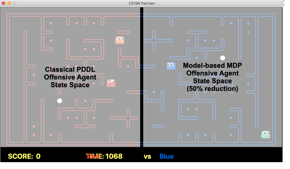
After implementing a basic MDP value-iteration agent, we faced the problem of huge state space due to which our agent is not able to perform 100 iterations within the required time-limit. In order to solve this problem, we considered the state space of the enemy’s territory only which leads to 50% reduction. This improved our computational speed and we were able to train the agent to learn a desirable policy.
In order to make our agent reach the enemy’s boundary, we used our classical PDDL approach. Hence, our strategy is to reach the enemy’s territory optimally and then turn into a model-based MDP agent so that we can utilize this approach for solving the limitations of our PDDL agent.
Trade-offs
Advantages
- Model-based MDP agent is able to learn a quite effective policy that avoids the ghost and tries to eat the food.
- Value iteration algorithm is able to show signs of convergence within 100 iterations which is computationally feasible if state space is chosen efficiently.
Disadvantages
- The above shown governing strategy works well on
tinyCapturewith less state space but couldn’t expand easily to other layouts. - Model-based MDP needs to store the Q-values of all states in order to decide a desirable policy that leads to updates that go beyond the provided time-limit.
- Value iteration algorithm convergence is not guaranteed within the provided iteration due to which we can never be sure about the effectiveness of the learned policy.
- It is difficult to implement a complicated decision tree as shown in PDDL Agent Offensive Strategy in our MDP agent due to the requirement of controlling flow via reward-shaping and Q-value initialization.
- Value iteration Model-based MDP approach is an offline-learning process and the game is extremely dynamic. Due to this, it is unlikely Value Iteration is going to work well without proper and effective heuristics in place.
Future improvements
- After properly training and utilizing a restricted state space approach, model-based MDP has the potential of finding rewarding policies.
- Decision trees can be created which fits the implementation of an MDP agent so that it is easier to map with the agent.
- With the reduced state space, iterations for the algorithm can be increased so that the learned policy is more effective.
- Ghosts anticipation can be added to the learning process and a heuristic-based strategy can be deployed which will eventually improve the learning process of our MDP agent.
Approach Four: Monte-Carlo Tree Search
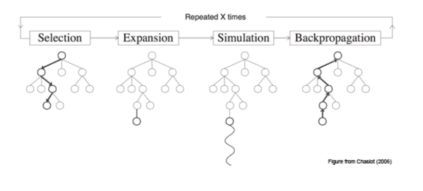
Monte-Carlo Tree Search (MCTS) is an online algorithm that can be used to explore a state space and react to positive and negative rewards. It uses simulations to infer the expected value of a state and is used in combination with Upper Confidence Bound (UCB) to balance the Exploration and Exploitation as it builds its search tree.
Implementation: myTeamMCTSAgent.py
Motivation
MCTS has a number of qualities that make it attractive for exploration in this Pac-Man competition. They are as follows:
- Online Algorithm: As we have a time constraint on calculation time, MCTS is an attractive option because it can terminate at any time and still return a useful result.
- Reward-based: This allows us to set the reward, rather than a goal. One of the difficulties experienced with Classical Planning and Blind/Heuristic search was picking the correct goal. There are many options for a goal, and they are situationally dependant. In contrast, the rewards have a more natural value as defined by the rules of the game. By being the reward-based, MCTS finds the best strategy for the current state, as well as the path. This is a significant motivation for trying this technique.
- State-space exploration: As MCTS generates a tree of states, we can easily update the other agents in the world to provide a more realistic state representation.
Implementation
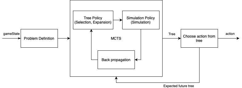
MCTS is defined by 4 key steps as defined in this diagram:
These were split into the following classes, to ensure substitutability of strategies:
Problem definition
This class contains domain-specific information required to generate the MCTS tree. Key methods include:
generateSuccessor
The method is responsible for generating the next state cause by taking an action. A number of key decisions were made here:
1. Apply action to the game state
2. Determine the expected action of the enemy and play this action.
3. Determine the expected action of teammate and apply the action.
4. Determine the expected action of the remaining enemy and play this action. This is done in the manner outline in step 2.
5. Record reward-related metrics about the state after the above action are applied.
Enemy Action
This contained basic logic to approximate the expected action of an enemy. When the enemy is a ghost, it will chase a Pacman within its territory. As a result, our agent would avoid getting into a situation where it would be eaten. When the enemy is a Pacman, it will run away from our ghosts, and attempt to escape back to its territory. As a result, our Pacman would rarely chase the enemy ghosts, as it realises it is not possible to catch them unless they move to a dead-end position, or our teammate can help block them. This had mixed results. A positive is that our agents wasted less time trying to catch agents they wouldn’t be able to reach. A negative consequence of this is enemies were generally left unobstructed, allowing them to roam our territory freely. A possible future improvement may be to reward our agents for having an enemy-free territory.
Teammate Action
This requires the teammate to store its expected path, as determined by the tree is generated. If this is available, the relevant action is applied when the current agent generates a successor. This was hugely influential on the performance and affects the agents in the following way.
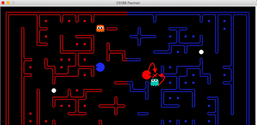
Food gathering As demonstrated below, by having access to the teammates planned actions, the agent can determine when the other agent is going to collect a given state before it and adjust its goal to accordingly. This was a powerful improvement as previously agents would make the exact same action, effectively reducing the teams capacity to a single agent.
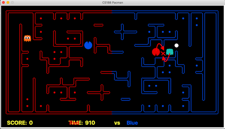
Enemy Chase The above improvement had a huge positive effect. Specifically, only a single agent would ever be motivated to try and trap/capture an enemy Pacman, because the other agent would realise it would not arrive at the enemy position first, and so would receive no reward. As a result, in a situation when the agent would previously have converged on an Enemy Pacman, one of the agents would now become indifferent, allowing the enemy to escape. To deal with this, both agents are rewarded of an enemy is trapped. This result in the following behaviour (we are the blue team).
Considering the teammate’s actions greatly expands the state space, so this was only considered when the teammate was within 7 maze distance from each other.
getReward
This determined the reward received for a state. Key features used were:
| Behaviour | Reward | Effect |
|---|---|---|
| Eating food | +.5 | Encouraged our Pacman to eat food |
| Enemy ghost eaten | +1 + 1*(number of food enemy carrying) | Rewards both agents when an enemy is eaten. This encourages agents too co-ordinate to eat an enemy. |
| Eaten by enemy ghost | - .5 - 1 * (number of food our agent is carrying) | Encourage our Pacman to avoid enemies |
| Score change | 1 * (score change relative to our team) | Encourages our agents to return food, and to prevent enemies Pacman’s escaping our territory with food. |
Tree Policy (Selection and Expansion)
This class is responsible for expanding the tree and choosing the node to be simulated. The Upper Confidence Bound (UCB) method was used for selecting children in nodes that were not yet fully expanded. This was chosen due to the elegant way it balances exploration and exploitation of the information in a tree, as discussed in lectures. While UCB proved effective, there were a number of other challenges that were faced here. State-space size: The the size of the state space is very large, which meant MCTS has to run for a greater amount of time before generating a useful result. The following effort was made to deal with this:
- Pruning: When generating new nodes, we check if the state represented by this node has already been seen in this path. We use a custom equality function to compare important state information, rather than everything in the state. If so, we mark this node as ‘dead’, which prevents it from being explored further. We then try to find a sibling node that is not ‘dead’. If this is not possible, we mark the parent node as ‘dead’, restart this iteration of the tree policy from the root. This was found to be highly successful in improving the usefulness of the tree, as it could concentrate on exploring novel states.
- Storing the tree: If the tree generated by an MCTS run is saved, this tree can then be built on in the agent’s next turn, provided this new state can be found in the tree. This allows MCTS to build more complete trees, by using its previous work as a starting point. This proved very helpful, as MCTS was then able to find very different goal states over successive runs. Unfortunately, this relies on being able to find the current state in the old tree. Unfortunately, a number of beneficial tool used to predict our opponent and teammate locations resulted in increased variability in the state seen between trees. This is something we would seek to investigate further in future work
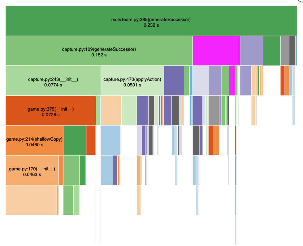
- Optimisation: By increasing the speed at which and we can iterate the MCTS algorithm, we can generate more complete trees in the allocated time. The following diagram shows the ~ 4x performance improvement that was achieved.
Original performance
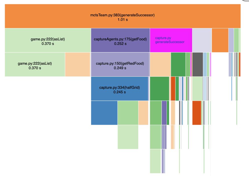
Improved Performance
Simulation Policy
The simulation aims to finds the expected value of a node/state that has never been visited before. When selecting a leaf node, simulation corresponds with finding the V(s’) component of the equation in the Back Propagation sections. A number of techniques were explored.
- Monte Carlo Simulation: This involves repeatedly selecting an action, generating a new state based on this action, until a terminal state or limit is hit. During this, the rewards received are tracked. This then provides a sample of the expected reward for reaching this state. This method was explored with different depth limits in our solutions. Unfortunately, the simulation step was quite expensive, as we were unable to find a suitable representation of the state faster than the ‘GameState’ object. Additionally, it was found that simulation introduced randomness into our tree. As we modelled Pacman as a deterministic game, this proved detrimental, as the simulation returned negative reward for states that could safely avoid these punishments. In our final solution, we decide not to simulated (simulate to depth 0), as we could instead use this computational budget to generate a bigger tree. As there is a maximum of 4 possible children for a node, this was feasible, but if there has been significantly more (e.g with non-deterministic modelling) this would not have been our strategy.
- Monte Carlo Heuristic Simulation: By providing a heuristic during the simulation phase, the simulation can be guided towards states that are likely to provide a reward. This was explored in a preliminary sense but was found to be reasonably nuanced. For example, if the heuristic encourages simulations toward food, it will completely avoid states that result in our agent being eaten, resulting in overly optimistic V(s’) values. Due to the 0 depth simulation decision, and the potential of a model-based approach (described below), this option was not explored further.
- Model-based approach: Using a model to estimate V(s’) was also explored. This involved using features and weights from approximate-Q learning to assign value to each state. This proved challenging, as the MCTS was very sensitive to the value provided by the model. This was found to influence MCTS to perform very similarly to whatever model was used, somewhat defeating the purpose of using MCTS. Future improvement may consider finding more sophisticated models through more advanced techniques.
Back propagation
Backpropagation is used to update the ancestors of a node, so they reflect the reward found in this node. A key challenge that was faced here was the backpropagation of negative rewards. When there were not yet sibling for a node with a negative reward, this negative reward would be propagated to the parent. This was a significant problem, as UCT (within the tree policy) was discouraged from further exploration of this parent, even when it had other suitable actions. A number of strategies were explored to deal with this issue:
- Discount factor: By adjusting the discount factor, the depth to which rewards were propagated can be an influence. This was not particularly effective for dealing with the problem described above. The discount factor similar to that recommended in assignment 4 was used.
- Learning rate: By adding a learning rate, a parent that has previously simulated a positive expected value, but then generated a child with a negative value, was able to retain some of its initial value. This was somewhat effective, but as the positive value can often be small (e.g 1 reward for eating food) and the negative rewards high (e.g -1 * all the food lost when the agent is eaten), the initial value was often overwhelmed. This was found to have adverse effects on other components of the tree. In our final solution, the learning rate was abandoned (set to 1).
- Generating all children: In non-deterministic trees, this problem is minimised, as when an action is taken, multiple child states are generated for that action. They are all assigned a value of 0, one of the children is simulated, and then backpropagation occurs as described in the first equation. If a negative reward is simulated, the effect of it is decreased by the other zero sibling nodes that are taken into consideration. Drawing on this, a deterministic version was created. This involved updates to the Tree policy, that were as follows:
- When reaching a node the is not yet fully expanded, for every available action, generate the child.
- For every child, set the value = 0 and ‘number of times visited’ = 0
- Choose a child for simulation, then follow the deterministic backpropagation algorithm outlined above. This change ensured that a parent would only have a negative value if all of its possible children were negative. This is well suited to the Pacman game, as the path is not affected by the sibling nodes, and the agent only needs to find a single positive path.
The following parameters were associated with backpropagation
| Parameter | Weight | Effect |
|---|---|---|
| discount | .9 | Agent acting mainly in a non greedy manner |
| learning_rate | 1 | Ensure nodes are updated completely with the current best value |
Critical Analysis
Advantages
- Does not require identification of goal states.
- MCTS allows agents to autonomous change from Pacman to Ghost as they determine is most beneficial.
- Can incorporate the expected behaviour of other actors in the world
Disadvantages
- Struggles with spares rewards. Without passing the previous tree forward it is often unable to reach states with rewards. We could not pass the tree forward due to enemy approximate tools, or when our agents were teammate aware. This proved to be extremely limited - as the agent could only effectively plan for reward located within approximate 7 steps from its current position.
Note Worthy Points
In our final agent, it was deemed that MCTS would defer to other planners when it recognised it had not found a reward (e.g the root node had a value of 0). As our existing agents where adept at escaping enemies and finding sparse rewards, these challenges were deferred to them in these situations, allowing MCTS to focus on its unique strengths of teammate awareness, and automatic offence/defence switching.
Future improvements
As mention in the above section, the primary area highlighted for improvement are:
- Exploring model-based simulation approach, particularly those which identify their own features
- Determining how to use previous trees when there is increased variability in the states (due to predicting enemy and teammate location and action).
- Optimising the Tree and simulation Policy to allow for bigger trees to be generated within the time limit
- More sophisticated teamwork that aims to find the state with the greatest reward for both of our agents
- Provide an incentive for an agent to keep enemies out of their territory, even if they can’t be eaten
Approach Five: Approximate Q-Learning
In this section, we will be explaining the usage of approximate Q-learning in our project. We first trained our model on several games with the baseline team and our PDDL agent team to get the best weights. Then, we used those weights for testing our agent’s performance. The results were satisfactory, but we applied this approximation to solve some of the limitations of our offensive PDDL agent that helped us to improve our game.
Implementation: myTeamApproxQLearningAgent.py
Approximate Q-learning Agent Architecture
In this section, we are going to explain the approximate Q-learning architecture for our agent. All of the components of the architecture are shown in the below image.
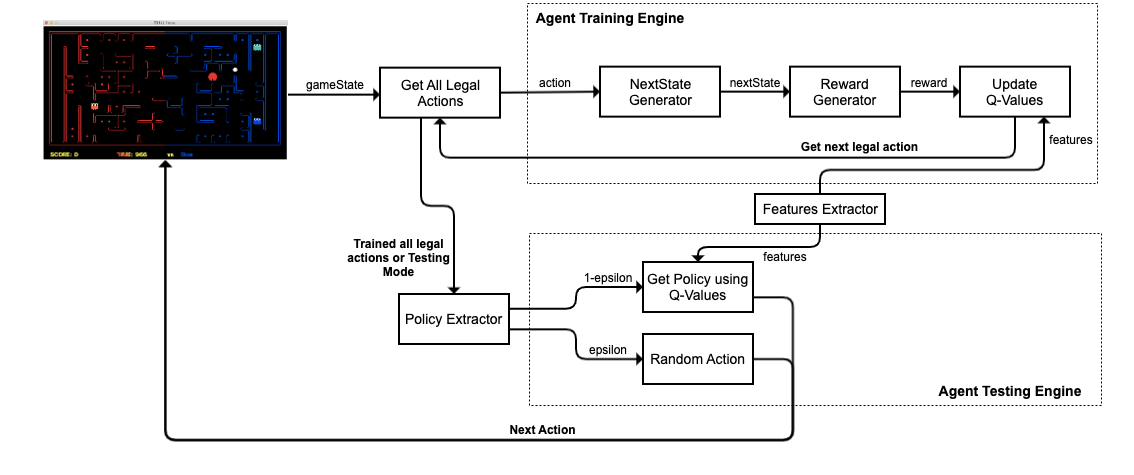
In this architecture, 2 main agent engines are used upon training and testing phases, as explained below.
Training Phase
Using the above architecture, we were able to train our agent so that weights can be learned depending upon situations in the game state. The steps of how an agent is trained can be stated as follows.
- Step-1: We first capture the game state and identify all the possible legal actions from the provided agent position.
- Step-2: For each action, we will update the weights for our Q-values. We first take the provided action and then generate the next state after applying that action.
- Step-3: Then, using the next state and current game state, we calculate the reward that is received by our agent for reaching that state.
- Step-4: We use our features extractor to get all the features for the current game state and provided action.
- Step-5: All of the previously calculated components are then used to update Q-values for the given state and corresponding action.
These training steps are then repeated until there are no more legal actions left. Then, we move to the testing phase to get the next action for our current game state.
Testing Phase
This phase is executed either in the training phase when all legal actions are explored or when the agent is not being trained anymore. The steps to identify an agent’s action in the testing phase can be stated as follows.
- Step-1: We first capture the game state and identify all the possible legal actions from the provided agent position.
- Step-2: Then, we pass all these legal actions to our policy extractor that either explore or exploit based on the provided
epsilonparameter. - Step-3.1: If the policy extractor decided to exploit, then we extract features from the feature extractor and use our trained Q-values to get the next best action that is providing maximum Q-value.
- Step-3.2: If the policy extractor decided to explore, then we choose random action from the provided legal actions.
Finally, we pass the next action to the gaming engine for execution on our agent. This will lead to a new game state, and then the training phase is repeated if it is enabled; otherwise, the agent’s move is extracted directly from the testing engine.
The training of our agent is done until all the provided training games are finished, and weights can be printed at the end of each game by using the below python function.
def final(self, state):
    "Called at the end of each game."
    # call the super-class final method
    CaptureAgent.final(self, state)
    print(self.weights)
Offensive Agent
In this section, we are going to explain the strategies and design patterns implemented for creating our offensive approximate Q-learning agent.
Motivation
The general idea for creating this agent is to implement aggressive and hostile behavior in our Pacman. Our objective is to make this agent responsible for crossing and entering into the enemy boundary and eat their food by surviving the ghost. The idea for exploring this technique is to solve some of the limitations of our offensive PDDL agent such as:
- PDDL Agent getting stuck: This was one of the major bottlenecks we faced with our offensive PDDL agent in which it gets stuck with our enemy agent. This situation usually arises because PDDL can’t anticipate future moves due to which it tends to move forward, thinking the enemy is not there. When the enemy is also there, then the planner decided to move backward. In such scenarios, our agent can’t explore other paths, and our offensive agent can’t perform any efficient moves.
- PDDL Agent timeout issues: There are some situations in which our offensive complicated decision tree is not able to compute the action effectively within the provided time-limit. In such scenarios, we lose the game due to 3 strikes.
These limitations can be solved using our Approximate Q-learning agent as it is pre-trained. Hence, it is computationally fast and also supports exploration, so have the ability to break out from the stuck state.
Implementation
As discussed in the architecture above, we have the training and testing phases for our agent. First, we train our agent by playing multiple games with the baseline team and over previous PDDL agent team to get the best weights which can be used for testing our agent’s performance.
We used the following features to enable basic approximating moves which are provided by our features extractor:
| Features | Description |
|---|---|
| closest-food | This feature is used to provide distance to the closest food for the agent’s position |
| bias | This feature is set to 1.0 so that we can capture bias weight for better performance |
| #-of-ghosts-1-step-away | This feature provides details of how many ghosts are 1 step away from the agent |
| eats-food | This feature is set to 1.0 if the agent eats the food so that weight can be trained upon this situation |
Next, we also implemented our custom reward generator that can be used to map rewards for our agent based on different situations:
| Situation | Reward |
|---|---|
| If Agent updated the score by collecting back the food | Reward = Difference of the score * 10 |
| If Agent can eat the food in the next state | Reward = 10 |
| If Agent encountered a ghost in the next state and died | Reward = -100 |
Then, we used the below bellman equation to update the weights for each feature.
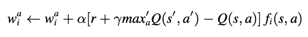
This is implemented in python using the below code.
  def update(self, gameState, action, nextState, reward):
    """
       Should update your weights based on transition
    """
    features = self.featuresExtractor.getFeatures(gameState, action)
    oldValue = self.getQValue(gameState, action)
    futureQValue = self.getValue(nextState)
    difference = (reward + self.discount * futureQValue) - oldValue
    for feature in features:
      newWeight = self.alpha * difference * features[feature]
      self.weights[feature] += newWeight
After weights are properly updated and trained, we can use these weights to get the corresponding Q-value of the provided state and action using below python code.
  def getQValue(self, gameState, action):
    """
      Should return Q(state,action) = w * featureVector
      where * is the dotProduct operator
    """
    features = self.featuresExtractor.getFeatures(gameState, action)
    return features * self.weights
Using these calculated Q-values based on the trained weights and features, we can get the action that is giving the best Q-value for exploitation or random action for exploration. After training for 50-100 games, our offensive approximating agent can perform well by dodging ghosts and eating food as required.
Governing-Strategy
The strategy of our offensive approximate Q-learning agent is to solve the above-stated limitations of our PDDL agent. These problems are solved by switching our PDDL agent into an approximating Q-learning agent by identifying the situation.
Solving PDDL Agent Stuck Problem
We have this intuition that approximate Q-learning can break out our PDDL agent from the stuck problem because of better anticipation of the ghost due to approximation with feature space and the ability to explore random paths. This strategy is implemented using the below steps:
- Step-1: Identify if our PDDL agent is stuck by storing all our agent actions in the queue and verifying the last 8 moves for any similar pattern.
- Step-2: If the agent is identified as stuck, then switch our agent to be an approximate Q-learning agent. We can switch agents using basic python object manipulations by having the agents pool, as shown below.
  def getApproximateModeAgent(self):
    self.AGENT_MODE = "APPROXIMATE"
    return self.agentsPool["APPROXIMATING_AGENT"]
- Step-3: Allow the agent to do either configured approximating moves like 5 or 10 moves or until any food is eaten.
- Step-4: If either of the above condition is fulfilled, then the agent is considered to be out of the stuck state, and we switch it back to be an offensive PDDL agent using a similar agents pool concept.
  def getAttackModeAgent(self, gameState):
      ....
      self.AGENT_MODE = "ATTACK"
      return self.agentsPool["ATTACKING_AGENT"]
      ....
We found this strategy of using approximate Q-learning quite effective, and it improved our winnings.
Solving PDDL Agent timeout Issue
The approximate Q-learning agent has weights that are pre-trained, and the features are calculated extremely fast. Hence, we saw that getting the next best action from our approximate Q-learning agent is extremely fast, and this can be utilized to solve any PDDL time-consuming action whenever it is taking more than the required time. The strategy can be stated as follows.
- Step-1: Enable a context-based timer to capture the execution time of our offensive PDDL agent action. This context-based timer is implemented using the python Signal library, as shown below.
@contextmanager
def time_limit(seconds):
    def signal_handler(signum, frame):
        raise TimeoutException("Timed out!")
    signal.signal(signal.SIGALRM, signal_handler)
    ...
- Step-2: With this function in place, we decided to set our custom time-limit of 0.9 seconds on the PDDL action decision.
- Step-3: If our PDDL agent takes more than 0.9 seconds, then the action is timed-out, and we switch our agent to be an approximate Q-learning agent.
- Step-4: Then, we get the next best action from our approximate Q-learning agent as it can be executed within the left 0.1 seconds.
Using these steps, we were able to capture time-outs before happening and provide an approximate action for just 1 move so that we can survive the hard time-limit constraint. Hence, this strategy helped us to place a fail-safe for our effective performing PDDL agent.
Trade-offs
Advantages
- Approximate Q-learning can be expanded easily to all possible layouts, thereby solving the major bottleneck of model-based MDP agent where we were struggling to train our agent on bigger state space.
- Approximate Q-learning can be trained offline, which enhances the ability of not getting timed out when playing games online. The trained weights are just multiplied with the corresponding feature space to approximate Q-values which provides a huge computational advantage.
Disadvantages
- Approximate Q-learning weights are extremely susceptible to the changes in the feature space due to which finding saturated weights is extremely difficult.
- Weights are also susceptible to situations. Due to this, weights are changed heavily when trained with a baseline team and when trained with our PDDL agent team.
- Exploring and creating a well-defined feature space that can generalize well in different situations is extremely hard. As a consequence, there is no convergence strategy for us to know if the found weights will work well in different scenarios.
Future improvements
- The approximate Q-learning agent is trained with a minimal feature space as the idea was not to create a full-fledged agent but to solve some of the limitations of our PDDL agent. This feature space can be expanded, and the agent can be trained again for more efficient results.
- Approximation of Q-values can also be enabled by using Deep Q-learning methods where weights and features can be learned simultaneously. This can be an excellent improvement for our approximating agent as the moves might be more accurate and weights will be more saturated.
Agent Strategies Improvements
In this section, we will be explaining different improvements which we have implemented on the top of our agents to improve their strategies and performance in the competitions. These improvements are not directly related to the approaches discussed before but they can be used together to improve the efficiency and solve limitations of our agents.
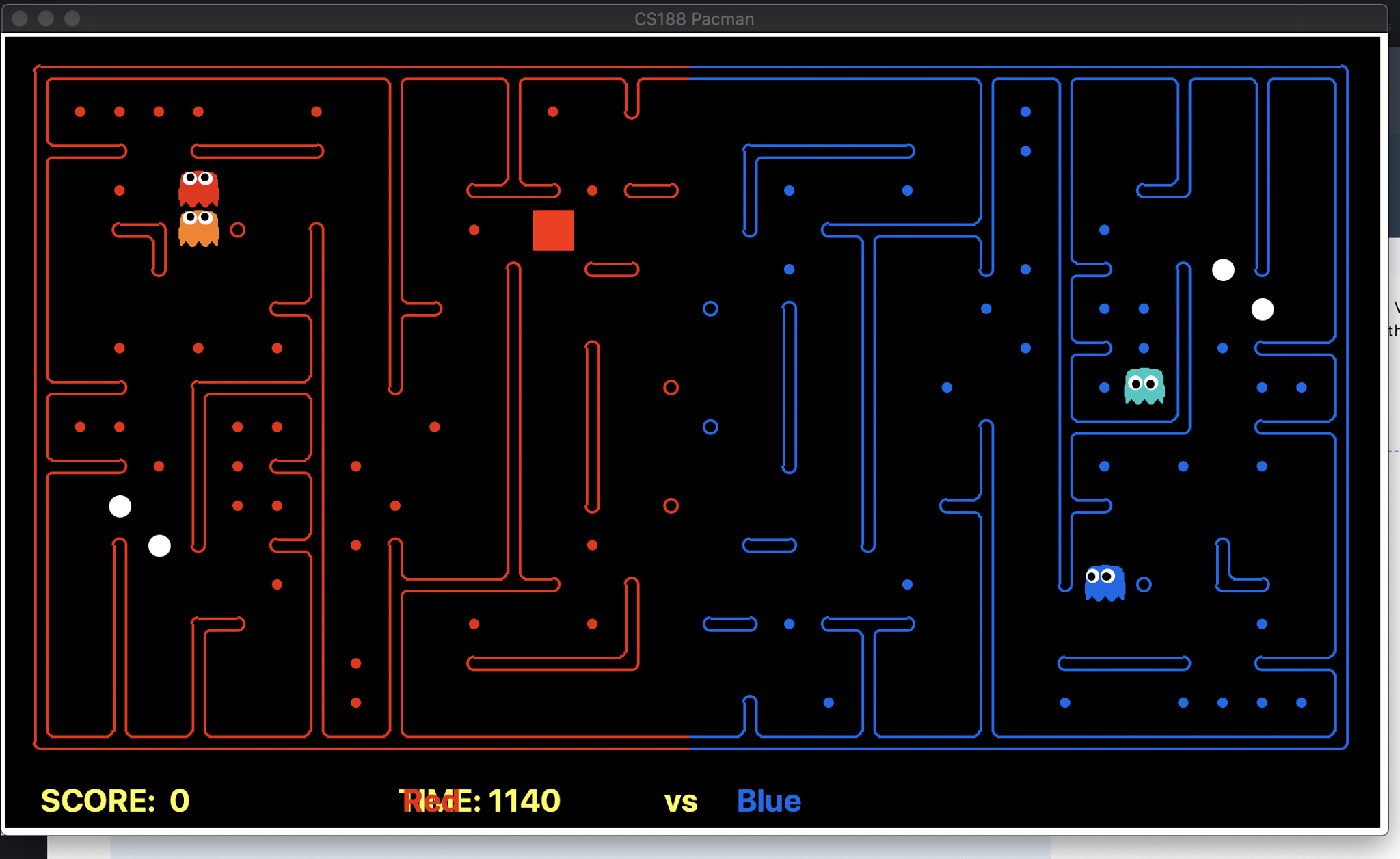
MaxFlow Algorithm: Identifying bottlenecks in the map
One of the defensive strategies we came up with was to find a bottleneck on the map, which covers a significant amount of food as well as the capsules. This idea popped up when we were testing our agent in one of the RANDOM maps. For example in the map below, if we placed our defensive agent at the red spot for the whole game without moving, it would deprive the enemy of all the foods and capsules covered by that entry point. These maps were frequently observed when we were testing our agents on RANDOM maps (We are the red team).
The hard part was the implementation of such an algorithm to acquire the bottleneck positions. We decided to use the Max Flow problem (through Ford-Fulkerson Algorithm) to detect the bottleneck positions. The implementation was creating an imaginary source node. Then attaching all the boundary positions to the source vertex with an infinite amount of flow (because the capacity is not of concern here), while all the other edges (legal adjacent positions on our side of the map) were given a capacity of 1.
Then we iterate over each of the food and capsule positions and extract the maxflow graph and find the vertex (farthest from the food/capsule) which when removed causes the food/capsule to be unreachable from the source. The vertex is the bottleneck position. This is done for all the food/capsule points, and the bottleneck position which covers most of the food, and all the capsules are extracted (the common vertex among them).
Bayesian Inference: Anticipating enemy positions
Relying on just being able to observe the enemy when it is 5 Manhattan distance is not optimal, in many situations we can estimate the enemy position giving us a better grasp of the state of the game. With this in mind, we decided to implement Inference with Time Elapse for anticipating enemy positions (inspired by UC Berkley Ghost Buster).
The idea behind this implementation is for each of the enemy agents we store a belief of where the agent is on the map based on our agent observations and state of the game. We make use of getAgentDistances and getDistanceProb which is provided. While the first function provides the noisy readings of the distance between our agent and the enemy agent, where the second function provides the probability of a noisy distance given the true distance. With the help of both these functions, we update our posterior (recent observations) based on the probabilities of the prior observations.
To further enhance the confidence of the anticipated positions we also include considerations of legal positions (a position which an agent can be in a map, i.e. not a wall), recent positions of eaten food and respawn positions (when our agent eats the enemy which we have access to through their agent state). At a particular state, the posterior probabilities are given higher weightage based on these considerations.
An example of this implementation is shown below with the probable positions acquired from our inference module. We can see at the time how confidently we can estimate the enemy positions. To acquire the positions, we take the position with the highest probability among all the positions for a given enemy (We are the red team).
Key takeaways
- Having access to a probable position of an enemy is a huge advantage and can be advantageous in many scenarios
- There is still a drawback, which is in huge maps if we don’t actually run into the enemy this could cause a huge misjudgment of the position (noisy distance may be well off) which could cause our agent to interpret the situation in a wrong way.
Handling blind spots for PDDL agent
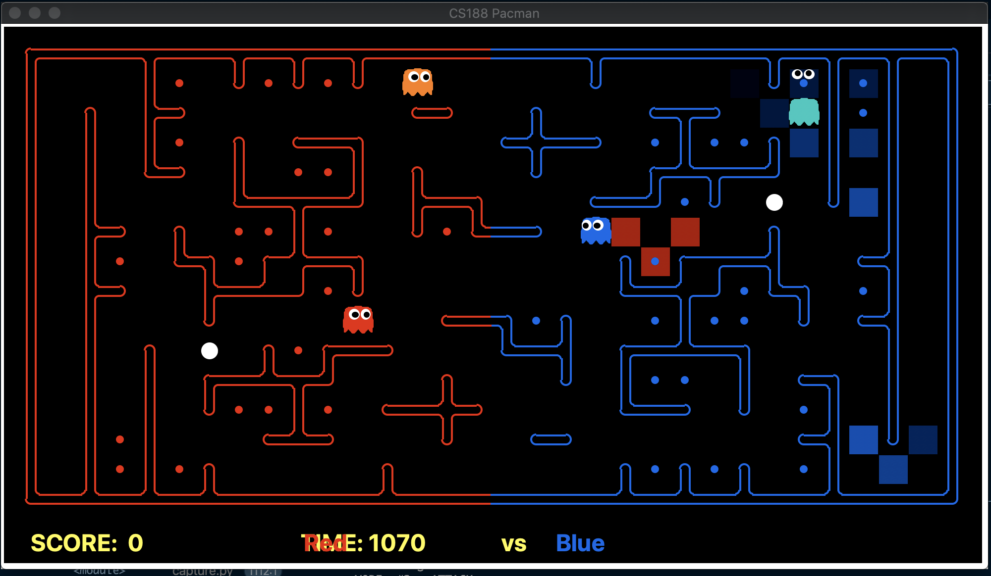
Classical planning suffers from a major drawback where it is not able to anticipate the next states as it only considers the current snapshot of the game. This exposes our PDDL agent to several blind spots in the game due to which we die at places that can be avoided. One of the blind spot situations is shown in the below image (We are the red team).
The above image clearly points out the spot in which our agent is allowed to move as the PDDL problem statement is not considering the fact that a ghost can also move to the same spot. As a result, in the next game state, our agent is killed by the ghost. A similar situation showing another blind spot is represented in the below image (We are the red team).
Again, we can see that according to the PDDL problem statement, Pacman is allowed to move to that spot since the ghost is currently 2 steps away. If we have executed our east move, then our agent will be killed by the ghost.
Hence, we overcome this problem of PDDL missing out blind spots by anticipating the ghost’s next moves and ensuring our agent is not allowed to move in those places. The idea is to capture if a blind spot is occurring which we can easily detect using the below python code.
  def checkBlindSpot(self, agentPosition, gameState, features):
      ghostsDist = [(ghost, self.getMazeDistance(agentPosition, ghost)) for ghost in ghostsPos]
      minGhostPos, minGhostDistance = min(ghostsDist, key=lambda t: t[1])
      if minGhostDistance == 2:
        if PDDL_DEBUG: print("!! Blind Spot - anticipate ghosts positions !!")
Once a blind spot is detected, the anticipated next ghost positions are identified and our PDDL agent is not allowed to move to those next positions. This improved our game and solved one of the limitations of classical planning.
Anticipating food depths using bottlenecks
Identifying the depth of the food was a very challenging and important task for us. Once we have anticipated food depths, then we can instruct our agents to behave in a cautious manner with respect to the depth of the food. In order to anticipate the food depth, we have expanded the use-case of our bottleneck identification using the Max-flow algorithm and used these bottlenecks to identify the depth of the food. This can be shown using the below image (We are the red team).
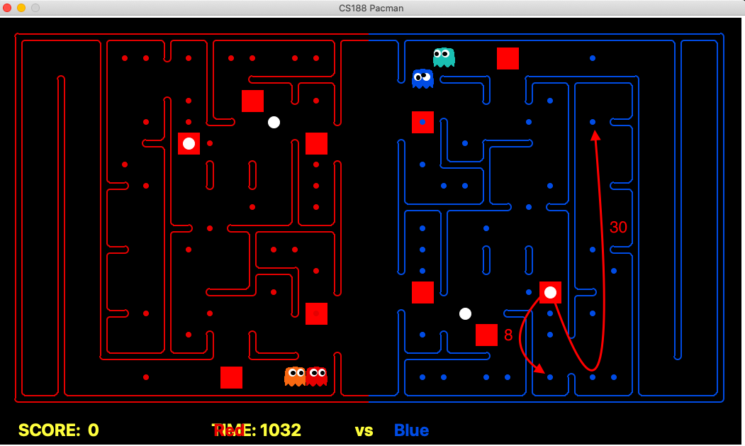
In order to calculate the depth, we use the following process at the starting of the game:
- First, we identify all bottlenecks in the map using the Max-Flow algorithm as discussed in the wiki above.
- Once bottlenecks are identified, we calculate the depth of each food inside the bottleneck by calculating the distance to eat that food and then coming back out from the bottleneck point. Hence, in the above example, for the food which is very deep inside the bottleneck, we take 15 steps to eat that food and then 15 more steps to come out from the bottleneck. So, the depth of the food will be 30.
- Then, identify food that is not covered by the bottlenecks and mark the depth of such food to be 0.
This process can be shown using the below python code.
  def getDepthPos(self, gameState, bottleNeckPos, offBottleNeckCount):
    ...
    # calculate depth of foods inside bottlenecks
    for pos, count in offBottleNeckCount:
      ...
      for food in coveredPos:
      ...
            foodDepth[food] = self.getMazeDistance(pos, food) * 2
      ...
    # put depth for the remaining food
    for food in foodsRemaining:
      foodDepth[food] = 0
    ...
    return foodDepth
Improving PDDL agent’s food selection using depth limits
After anticipating the depth of the food as shown in the above section, we instructed our agent to consider these depths while exploring the food. In order to do this, we introduced the concept of the depth limit for our agent. Since the limit for depth to be explored cannot be generalized, we placed this logic only for the capsule-based maps in order to improve the food selection process for our PDDL agent. The process works as follows:
- Initially, if the map is having capsules, the depth limit is set to 2. As per this depth limit, our offensive agent is not allowed to eat the food which is having depth > 2. This ensures that our agent doesn’t die at the beginning of the game exploring deeper regions.
- Once any capsule is eaten or food of depth 0-2 is collected back home, we allow our agent to explore deeper foods now by removing the depth limit.
This process is not dynamic since it is not easy to judge and generalize the idea of limits on depth on all random layouts. The idea can be shown using the below game situation (We are the red team).
It can be seen that our offensive agent decided to eat food with a depth of 2 at the beginning of the game which helped our agent to avoid deeper foods. Due to this, the deeper foods are initially skipped until the capsule is eaten or all the food with depth <=2 is collected back home. This enhances our food selection process and increases our chances to win the game.
Experiments and Evaluation
Final Submitted Agent
In this section, we will explain our agent that will be submitted as our final submission for the competition. In our final agent, we have utilised multiple approaches depending upon different situations to improve the performance and tackle limitations of our implemented scenarios. We have combined the strengths of the following approaches in our final agent:
- Classical Planning (PDDL) as our default offensive and defensive agent.
- Monte-Carlo Tree Search for an offensive and defensive agent in the situation of no capsules on the map.
- Approximate Q-learning for an offensive agent to break the stuck state and get next move if the time limit is reached.
Implementation: myTeam.py
Motivation
The idea is to create one master agent that can control when to use what technique. Using this approach, we can make our defensive PDDL agent turn into an offensive PDDL agent, take help from Monte-Carlo agent to get next actions and identify points where approximate Q-learning agent can be useful. This can help us to overcome the limitations of the different approaches as we will be able to combine the strengths of our agents and use them depending upon the situation.
Governing-Strategy
In this section, we are going to explain the governing strategy of our final submitted agent briefly. It is based on the idea of switching agents depending upon the situation, as explained in the below decision tree.
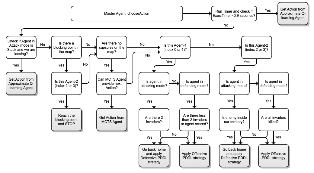
This strategy is executed as soon as our agent requires the next action. First, we start our time-limit engine with a limit of 0.9 seconds. As soon as the time-limit is reached, we stop the execution of our code and take help of approximate Q-learning agent to get the next action as it hardly takes 0.01 - 0.09 seconds to answer based on the current game state. If we are within our time-limit, then following decision tree is executed.
- We first check whether the agent in attacking mode is in a stuck state. Once the stuck state is captured, we identify whether we are winning the game or not. If we are winning, then we don’t let our agent come out from the stuck state as we know that we will be stuck with one of their agents. If we are not winning, then we transform our agent into approximate Q-learning agent who executes its governing strategy. This agent combines the strength of exploration-exploitation to come out from the stuck state.
- Otherwise, we identify if there is any blocking point in the map using Max-flow algorithm as discussed in the Agent strategies improvements wiki. Any point is considered as the blocking point in the map based on the criteria shown in the table below. If any of the criteria are met, then our defending agent goes to the blocking point and stops there throughout the game:
| Point Description | Is blocking point? |
|---|---|
| If the map is no capsule and the point is covering 70% of the food | Yes |
| If it is a capsule-based map and the point is covering 60% of the food | Yes |
- Next, we identify if there are no capsules in the enemy’s territory. In such a situation, we don’t have any strong Offensive PDDL strategy when the ghost chases Pacman as we always run back home if there are no capsules left in the map. So, we transform our agent to Monte-carlo agent and check if it can give us any valid action based on the criteria as described in Monte-Carlo agent noteworthy points. If the agent can give us the next action, then it is executed. Otherwise, the decision flow is continued.
- Now, we apply our strategy by marking agent with index 0 or 1 as Agent-1 and index 2 or 3 as Agent-2. Our default offensive agent is Agent-1. If Agent-1 requires next action, we undertake the following decisions:
- By default, this agent works on the discussed Offensive PDDL strategy.
- If there are 2 invaders in our territory, then we use our offensive PDDL strategy to make our agent come back and turn it into a defensive agent which is then going to apply Defensive PDDL strategy. Our agent-1 will stay defensive until invaders are reduced and then it turns into an offensive PDDL agent again.
- Similarly, our default defensive agent is Agent-2. If Agent-2 requires next action, we undertake the following decisions:
- By default, this agent works on the discussed Defensive PDDL strategy.
- As soon as this defender can kill all invaders in the territory, we turn this agent into an offensive agent which is then going to apply Offensive PDDL strategy. Our agent-2 will stay offensive until an enemy has entered in our territory. Once the invader is identified, we turn this agent back to a defensive agent.
Implementation
To implement the above shown governing strategy, we used the concept of python classes and objects to control the execution flow. We are below the structure for all our agents.
def createTeam(firstIndex, secondIndex, isRed,
               first='MasterAgent', second='MasterAgent'):
 """ Function for team creation """
 ...

class BaseAgent(CaptureAgent):
  """ Helper functions for all Agents """
  ...

class MasterAgent(BaseAgent):
  """ Master Agent to initialise and control all agents """
  ...

class OffensivePDDLAgent(BaseAgent):
  """ Classical PDDL offensive agent """
  ...

class ApproxQLearningOffense(BaseAgent):
  """ Approximate Q-learning offensive agent """
  ...

class DefensivePDDLAgent(BaseAgent):
  """ Classical PDDL defensive agent """
  ...

class MctsAgent(BaseAgent):
  """ Monte-Carlo Offensive/Defensive agent """
  ...
Now, in order to take agents, depending upon the situation as described in the decision tree, we are maintaining an agents pool as shown below, where all these agents are placed as hot agents and can be directly picked out without re-initialising their registerInitialState function.
    self.agentsPool = {
      "ATTACKING_AGENT": attackingAgent,
      "DEFENDING_AGENT": defendingAgent,
      "APPROXIMATING_AGENT": approxAttackAgent,
      "MCTS_AGENT": mctsAgentInstance
    }
Trade-offs
Advantages
- The use of a decision tree and combination of techniques allowed specialisation within the agent, resulting in improved performance.
- Approximating moves using Q-learning is extremely helpful as it is able to overcome PDDL’s strict problem-based nature. Using approximation, our agent is able to take a higher risk which can be really rewarding and also helped us to make our agent come out of the stuck state.
- Approximate Q-learning uses pre-trained weights. This helped us to use an approximation of the move when our allotted time runs out as it takes 0.01-0.09 seconds for getting the results. Due to this, we were able to set 0.9 seconds as the time limit for the execution of our logic.
- Combining PDDL with MCTS proved to be most beneficial, as PDDL can quickly determining paths in sparse reward situations. In contrast, MCTS can determine its own goals (via the rewards set) and produce more nuanced behaviour in non-sparse reward situations.
- PDDL is fast and can act as a fall back after MCTS has failed to produce a satisfactory path. If PDDL were slower, this would create a much more challenging situation in which we would have to identify which approach was most appropriate before running them.
Disadvantages
- PDDL offensive-defensive switch behaviour is not able to work well when the enemy’s agent is stuck at the boundary due to which our offensive agent decides to be defensive due to heavy invader but then turn into offensive as invaders are reduced. This causes our agent to be in the stuck state because of the behaviour changes at the critical points in the map. Similarly, our defensive agent turns into an offensive agent if an enemy enters the territory and it can also cause the same problem if the enemy is stuck at the boundary.
- Approximate Q-learning is not able to consider the depth of the food while approximating the next move. As a result, our agent is able to escape stuck state but might die trying to eat the food which is in greater depth. Moreover, there is 0.05
epsilonexploration while approximating move which might not work in our favour if our agent decided to explore a path that takes him to the ghost. - There appears to be some communication issue between MCTS and PDDL, as in some cases the advocate markedly different strategies. As a result, instead of sticking with one not ideal strategy, it swaps rapidly between the two, effectively using no strategy at all.
- The use of multiple strategies increases the complexity of the agent, resulting in more complex debugging and behaviour appraisal. The team found it very challenging at a time to determine if poor behaviour was due to bug/flaws, or just bad luck in a specific case. The empirical model assessment was increasingly required, as seemingly simple improvements tended to have flow-on effects.
Future Improvements
The team would be particularly interested in exploring methods that use the agents collaboratively, as there appears to be a great opportunity and complexity in this space. While some initial efforts were made in MCTS, PDDL and Q-learning, the team would love to take this further. Additional, a large amount of time was spent identifying features and handling specific cases. The team would be very interested in implementing more advanced reinforcement learning such as deep neural nets, to investigate if this could assist in combating these issues.
Evolution and Experiments
In this wiki, we will be evaluating and explaining the performance of all our attempted agents that we have implemented using different approaches discussed in the Design choices section of the wiki. First, we will show the performance of our different agents with the baseline team and competitions results. Then, we will discuss the evolution of different approaches by critically analysis their strengths, weaknesses and competition performances. Finally, we will analyse the improvements implemented in our final submitted agent, which is followed by a comparison of all our agents.
Agents performance
Performance with BaseLine Team
To have a baseline to compare with, we ran all our agent implementations against the baseLineTeam on 10 RANDOM maps. The Seeds for the Maps were {2401, 1730, 6725, 70, 6864, 6641, 7315, 5365, 1749, 1979} which were randomly generated.
| Team | Win | Tie | Lost | Score Balance |
|---|---|---|---|---|
| BFS and A* Agent | 9 | 1 | 0 | 84 |
| PDDL(1 offensive & 1 defensive) | 8 | 2 | 0 | 167 |
| Model-based MDP Agent | 0 | 10 | 0 | 0 |
| MCTS | 0 | 10 | 0 | 0 |
| Approximate Q-learning Agent | 1 | 8 | 1 | 0 |
| PDDL (Dual switching mode) | 10 | 0 | 0 | 242 |
| PDDL + Q Learning | 10 | 0 | 0 | 240 |
| Final Implementation (MCTS + PDDL + Q Learning) | 10 | 0 | 0 | 239 |
We can see from the above results that PDDL agents are extremely powerful with the ability to generalise well on different random layouts. Hence, we combined the techniques such as approximate Q-learning and MCTS using PDDL as our core engine to improve our performance and solve different limitations of our PDDL agent.
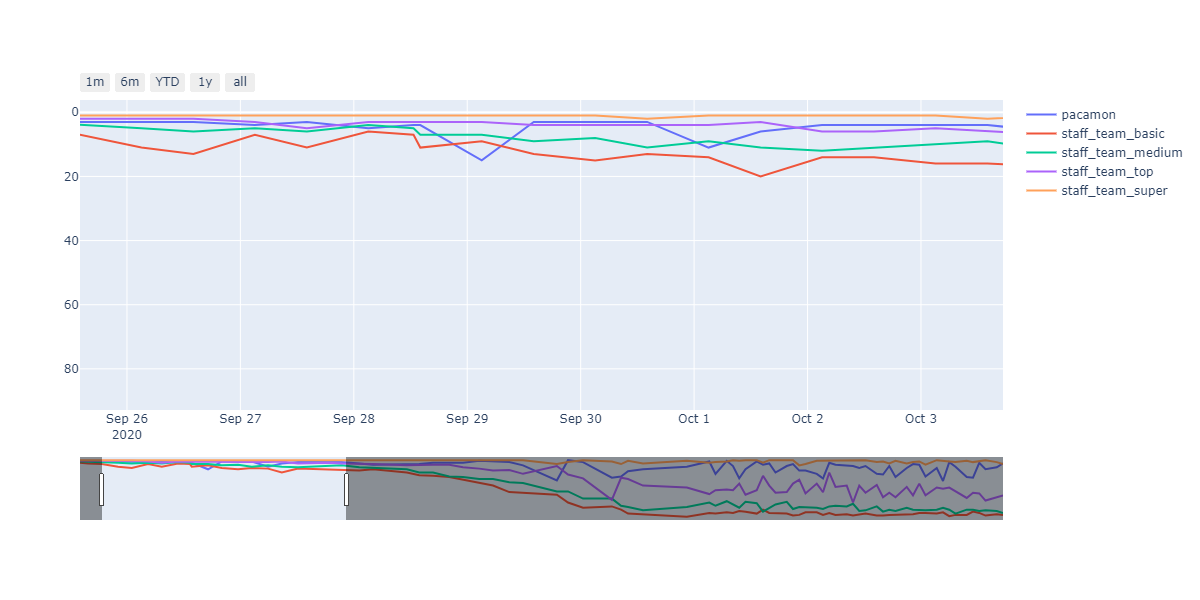
Performance in the Competitions
In this section, we will be summarising the pre-competition and preliminary results for our different submitted agents. The pre-competitions started from 09/24 20:37, and we submitted our first agent for 09/27 03:04 run. The results of how our different agents performed throughout the competitions can be summarized using the below table and plot.
| Team | Total Games | Points | Win | Tie | Lost | Win(%) | Tie(%) | Lost(%) |
|---|---|---|---|---|---|---|---|---|
| PDDL(1 offensive & 1 defensive) | 1920 | 3679 | 1285 | 109 | 526 | 66.927 | 5.677 | 27.396 |
| PDDL (Dual switching mode) | 1910 | 4229 | 1387 | 68 | 455 | 72.618 | 3.560 | 23.822 |
| PDDL + Q Learning | 1802 | 4006 | 1322 | 40 | 440 | 73.363 | 2.220 | 24.417 |
| Preliminary | 704 | 1485 | 489 | 18 | 197 | 69.460 | 2.557 | 27.983 |
| Final Implementation | 7012 | 14623 | 4802 | 217 | 1993 | 68.483 | 3.095 | 28.423 |
| Total | 13348 | 28022 | 9285 | 452 | 3611 | 69.561 | 3.386 | 27.053 |
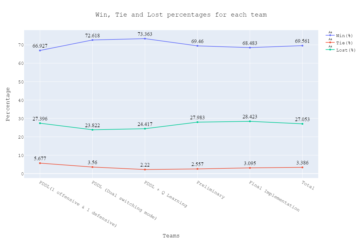
We can see from the above results that we have maintained a consistent average win rate of more than 65% throughout the competition runs. This is again shown with the results of our preliminary agent with the average win rate of 69%. As the competition went ahead, the teams started getting stronger. However, our win rate with our final implemented agent is still above 65% (last recorded 10/26 10:05), which clearly outlines the strength and stability of our implemented techniques in our final submitted agent. The results from the preliminary competition (10/15 02:09) can be stated as follows. We were able to secure the 11th rank with 489 points.
| Position | Team | Points | Win | Tie | Lost | TOTAL | FAILED | Score Balance |
|---|---|---|---|---|---|---|---|---|
| 7 | triplez | 1566 | 513 | 27 | 164 | 704 | 0 | 6378 |
| 8 | wuhu | 1526 | 504 | 14 | 186 | 704 | 86 | 10084 |
| 9 | shake-a-leg | 1516 | 497 | 25 | 182 | 704 | 3 | 3781 |
| 10 | silly-ramen | 1507 | 492 | 31 | 181 | 704 | 0 | 5280 |
| 11 | pacamon | 1485 | 489 | 18 | 197 | 704 | 1 | 5061 |
Evolution of the approaches
In this section, we will be critically analysing different approaches that we have attempted and implemented in this project. We will try to outline the strengths and weakness of each approach using situations from our self-attempted game and pre-competition replays.
Approach 1 - BFS and Astar Agent
In this section, we will be explaining and discussing the performance of our BFS and A* Agent approach. We used these agents to explore the advantages and disadvantages of search algorithms. We have drafted a more straightforward offensive agent that can exploit the generate successor available in gameState. We have also explored the strategies that were required in general by defensive agents. Both the offensive and defensive strategies are limited by the decision of goal state since the goal state needs to be clearly defined at the beginning of the problem definition. Hence we ventured to the other algorithms that could provide more flexible goal state assignment.
Strength: Our offensive agent was able to eat capsule and avoid enemy without explicitly setting these as goal states. Also, our defensive agent can detect the territory breach, track the positions of eaten food.
We have implemented the strategy for defensive agents on the blue team here(light blue).
Weakness: For defensive goal position heavily relies on the governing strategy. For offensive agent, increasing the threshold for the score can lead to a significant increase in the node expansion in the search algorithms.
| Heuristic Agents (1 offensive & 1 Defensive) | Win | Lose | Tie |
|---|---|---|---|
| staff_team_basic | 8 | 2 | 0 |
| staff_team_medium | 7 | 2 | 1 |
| staff_team_top | 1 | 9 | 0 |
| staff_team_super | 1 | 9 | 0 |
We have not used this algorithm in the final agent since behind the hood, PPDL also uses the search algorithms to find the optimal paths. We had built a fully functioning PPDL offensive and defensive agent in parallel and further enhancing A*, or BFS algorithm would have led to redundant work. We have passed on some of the governing strategies to the other approaches and didn’t explore these agents further.
Approach 2 - Classical Planning
In this section, we will be explaining and discussing the performance of our Classical Planning (PDDL) based Agent approach. Out of a lot of agents, Classical Planning was the easiest to get started with. Most of the work was in defining a clear Offensive and Defensive agent domain PDDL. The standalone PDDL (offensive & defensive) was our initial agent deployed for running in the pre-competitions. We can see that using a clear PDDL domain formulation along with ad-hoc PDDL problem formulation, we were performing decently throughout the initial stages. We were between staff_team_top and staff_team_medium mostly with beating staff_team_top during the ending stages of PDDL testing with new heuristics. This can be observed in the image below.
Strength: With minimal logic coding required, the agent was able to figure out the optimal path of dodging enemy and getting to the capsule which is returned by the planner. The only factor changing in a PDDL problem is the goal. For example, in the image below we can see when we run into close proximity of a ghost, we try to run towards the capsule but a path might not always emerge, this is where our agent figures out the optimal path through the planner (We are the red team).
Weakness:
- Due to the drawback of not being able to anticipate steps ahead, our agent always gets cornered in positions where the food is deep in a corner which has the same exit as the entrance. This can be seen from one of the replays from the competition in the illustration below (We are the red team).
- Another weakness which is prominent among the games the agent plays is it gets in a stuck situation. This happens because the agent reformulated the problem at every step which brings it back to the same position as the enemy would move in the same direction to chase you. This is illustrated below (We are the red team).
Approach 3 - Model-based MDP Agent
In this section, we will be explaining and discussing the performance of our Model-based MDP agent approach. We are using this agent to test offensive strategy with MDP and the performance was not good enough to actually use this approach in our final agent.
Strength: With proper rewards shaping, the agent was able to dodge ghost and eat food as shown in the game below (We are the red team).
Weakness: Even after efficient policy learning, our offensive agent is not able to defeat the baseLine team due to the rewards sparsity problem. This leads to Q-value being 0 for all actions leading to the below shown stuck state (We are the red team).
Due to the above problem, this approach was not able to generalise well on different layouts and couldn’t win any of the games with baseline team. Hence, we haven’t pursued this approach further.
Approach 4 - MCTS
In this section, we discuss the performance of Monte-Carlo Tree Search.
Strengths: MCTS can perform well when there are rewards close to the agents. It is particularly suited to agent co-operation, as demonstrated in the Monte-Carlo wiki.
Weakness:
Unfortunately, incorporating agent co-operation comes at the cost of using pervious search trees. As a result, MCTS cannot explore the search space far enough to produce any action on non-trivial maps. This is why, without the support of other methods, it loses to the baseLineTeam, as it has to falls back to random behaviour, never getting far enough from the start position. This is demonstrated below as MCTS (blue), cannot systematically move away from the start position.
Approach 5 - Approximate Q-learning
In this section, we will be explaining and discussing the performance of our Approximate Q-learning agent approach. Using the features and training weights as explained in the wiki, our offensive agent is able to beat the baseline team in some of the matches where we have used the same defensive reflex agent to evaluate the performance correctly.
As per the results shown in the top of wiki, we concluded that standalone approximate Q-learning needs a whole lot of work on the features space to learn the right weights in order for it to perform well. In addition to this, we realised that the strength of approximate Q-learning is to use features and learned weights to perform nice approximation, which can be used to solve our agent’s problem to remain in the stuck state throughout the game as shown in the PDDL agent and MDP agent approaches.
We can show this using the below game where our PDDL agent was stuck as the ghost was not moving. In such a situation, approximate Q-learning is able to help PDDL agent to come out of the stuck state quite efficiently (We are the red team).
Before adding this improvement to our PDDL agent, we were not able to beat the top team as per the results from 10/04 15-04.
| Position | Team | Points | Win | Tie | Lost | TOTAL | FAILED | Score Balance |
|---|---|---|---|---|---|---|---|---|
| 7 | staff_team_top | 419 | 134 | 17 | 59 | 210 | 0 | 898 |
| 8 | pacamon | 413 | 135 | 8 | 67 | 210 | 10 | 1364 |
After adding this approximation if our PDDL agent is stuck to the pre-competition, our rankings improved as per the results from 10/07 04-04.
| Position | Team | Points | Win | Tie | Lost | TOTAL | FAILED | Score Balance |
|---|---|---|---|---|---|---|---|---|
| 5 | pacamon | 498 | 165 | 3 | 48 | 216 | 5 | 1952 |
| 6 | triplez | 485 | 160 | 5 | 51 | 216 | 0 | 1665 |
| 7 | house-tangaryen | 482 | 156 | 14 | 46 | 216 | 1 | 2369 |
| 8 | staff_team_top | 463 | 151 | 10 | 55 | 216 | 0 | 1097 |
Below pre-competition ran on 10/08 04-04 shows one of the matches with staff-top team on RANDOM5692 which we were able to win because our PDDL agent is able to get out of the stuck due to the approximation suggested by approximate Q-learning (We are the red team).
Testing approaches
As the teams began to increase for the competition the layouts and games played at different layouts started to decrease. And evaluating agent performance of generalising was hard to test. To cope with this issue we developed a testing script which would run our agent across RANDOM map seeds to test (against old agents) and store the logs and output for the test run. The implementation can be found here.
For testing, we used the following logic as shown below.
for i, SEED in enumerate(seeds):
    for TEAM_BLUE in teams:
        proc = Popen(f'python capture.py -r {TEAM_RED} -b {TEAM_BLUE} -l RANDOM{SEED} -q'.split(),
                            stdout=myoutput, stderr=subprocess.PIPE, universal_newlines=True)
        proc.wait()
        write_to_file.....
Final Submitted Agent
In this section, we will discuss the performance improvements after combining the above techniques for solving different limitations. We will also explain how enhancements to the above techniques helped us to improve our rankings in the competition.
PDDL Agent improvements with offensive-defensive switch
We have enhanced our PDDL agent to switch their behaviour depending upon the strategy as discussed in the above wiki. Before adding the offensive-defensive switch behaviour, we were not able to beat the staff-medium team in the pre-competitions as shown in the results below from 10/01 03-04.
| Position | Team | Points | Win | Tie | Lost | TOTAL | FAILED | Score Balance |
|---|---|---|---|---|---|---|---|---|
| 9 | staff_team_medium | 262 | 84 | 10 | 86 | 180 | 0 | -362 |
| 10 | funpacman | 250 | 78 | 16 | 86 | 180 | 0 | -278 |
| 11 | pacamon | 246 | 81 | 3 | 96 | 180 | 15 | -709 |
After adding the offensive-defensive switch behaviour, we were able to beat both staff-medium and staff-top teams in the pre-competitions as shown in the results below from 10/02 14-04.
| Position | Team | Points | Win | Tie | Lost | TOTAL | FAILED | Score Balance |
|---|---|---|---|---|---|---|---|---|
| 4 | pacamon | 416 | 136 | 8 | 46 | 190 | 4 | 1957 |
| 5 | awful-go | 409 | 135 | 4 | 51 | 190 | 0 | 675 |
| 6 | staff_team_top | 379 | 124 | 7 | 59 | 190 | 0 | 695 |
This switch is extremely effective as our defensive agent is able to turn into an offensive agent and collect food back if there is no invader in our territory. This can be shown using one of the replays with staff-top team on RANDOM7814 map from the pre-competition 10/02 14-04. It can be seen from the demo that one of our offensive agents decided to turn back and be a defensive agent as soon as the enemy entered our territory (We are the red team).
Identifying blocking points in the map
In this improvement, we have used the Max-Flow algorithm to identify bottlenecks in the map as discussed in the improvements wiki. After identifying the bottlenecks which cover a certain threshold of the food with capsules, we instruct our defensive PDDL agent to reach the bottleneck point and stay there throughout the game.
Using this improvement, we were able to defeat staff-team-super on the pre-competition ran on 10/11 03-04 as the map chosen for the competition was having a bottleneck that covers both capsules and certain threshold of the food. The results from that pre-competition were as follows.
| Position | Team | Points | Win | Tie | Lost | TOTAL | FAILED | Score Balance |
|---|---|---|---|---|---|---|---|---|
| 1 | pacamon | 196 | 63 | 7 | 4 | 74 | 1 | 692 |
| 2 | pac-superman | 193 | 64 | 1 | 9 | 74 | 0 | 701 |
| 3 | silly-ramen | 192 | 63 | 3 | 8 | 74 | 0 | 855 |
| 4 | staff_team_super | 187 | 61 | 4 | 9 | 74 | 0 | 609 |
This bottleneck approach is extremely powerful for the maps with bottleneck points. This can be shown using one of the matches with staff-team-super that ran on 10/11 03-04 RANDOM3241 map which shows the effectiveness of this strategy. It can be seen that our defender is able to trap both super agents by identifying accurate bottleneck, due to which we were able to win this game (We are the red team).
Using MCTS agent when there is no capsule on the map
MCTS was introduced to help our agents take calculated risks and more aggressively explore the enemy territory. MCTS is run when there are no longer capsules that our team can eat. MCTS attempts to identify reward receiving behaviour, and if it is unable to find any, signals the agent to use the standard decision logic. This allows us to exploit the strengths of MCTS in non-sparse reward situation while avoiding MCTS problematic behaviour in sparse situations. One of its strength is the ability to anticipate enemy chase behaviour, allowing it to take calculated risks. This can be seen in the behaviour of the top left blue agent, as it can determine the exact depth to move to, without becoming trapped. This improved the existing behaviour, which was to immediately return home when nearby agents were spotted. This logic was used as PDDL was unable to simulate the enemies chase behaviour (We are the blue team).
Weakness Unfortunately, if MCTS builds a plan using anticipated behaviour that is incorrect, the results can be poor. For this reason, we have kept anticipation logic as simple as possible (enemy ghost will chase nearby Pacman).
 |
 |
|---|---|
| Enemy acted as anticipated, our agent safely collects food (We are the blue agent). | In the same location with a different enemy, our agent gets stuck (We are the red agent). |
Over the ending period of the pre-competitions on our final agent deployment run, we managed to overtake staff_team_super in the runs with the help of MCTS as shown in the below table (25/10/20 15:00 Run).
| Position | Team | Points | Win | Tie | Lost | TOTAL | FAILED | Score Balance |
|---|---|---|---|---|---|---|---|---|
| 5 | triplez | 412 | 136 | 4 | 36 | 176 | 0 | 2561 |
| 6 | pacamon | 410 | 135 | 5 | 36 | 176 | 0 | 1165 |
| 7 | staff_team_super | 405 | 134 | 3 | 39 | 176 | 0 | 1553 |
In one of the matches from the run above (pacamon vs staff_team_top on RANDOM1765) we can evidently see MCTS at work (We are the red team). In the situation below being chased by a ghost, our initial agent would have run back home because of the lack of capsules but our final agent with the help of MCTS evaluates that devouring that 2 food would hand us the win while on the way back home without being eaten by the enemy.
Summary and model comparison
In this section, we will summarise the above discussion, comparing the performance of different models in specific situations. We will follow the below-shown rating scheme to evaluate the different approaches we have implemented using our agents.
| 1 | 2 | 3 | 4 | 5 |
|---|---|---|---|---|
| Very Poor | Poor | Average | Good | Very Good |
| Very Low | Low | Average | Good | Very High |
| Very Slow | Slow | Average | Fast | Very Fast |
The comparison of different approaches based on 5 different criteria is summarized using the table below.
| Technique | Sparse Rewards | Avoids Manual update of goal states | Requires Feature Selection | Future Anticipation | Execution Speed |
|---|---|---|---|---|---|
| BFS and A* Agent | Very Good | Average | Average | Very Poor | Very fast |
| PDDL (1 offensive & 1 defensive) | Very Good | Very Poor | Average | Very Poor | Very fast |
| Model-based MDP Agent | Poor | Good | Low | Poor | Very slow |
| MCTS | Poor | Very Good | High | Very Good | Slow |
| Approximate Q-learning Agent | Average | Good | Very High | Average | Very fast |
| PDDL (Dual switching mode) | Very Good | Very Poor | Average | Very Poor | Very fast |
| PDDL + Q Learning | Very Good | Poor | High | Poor | Very fast |
| Final Implementation (MCTS + PDDL + Q Learning) | Very Good | Good | High | Good | Average |
As per the above table, we can infer the following observations:
- Sparse Rewards: This is used to categorize approaches based on their ability to find the best distant food. We can observe that search algorithms and PPDL, which used a search algorithm in the background are good at finding the optimal path to distant food. However, MCTS and MDP are not that great at detecting distant food.
- Avoids Manual update of goal states: This is used to categorize the approaches based on the flexibility they provide in avoiding the manual decision tree generating. MCTS is best in avoiding this since it works based on the simulation and reward strategies.
- Requires Feature Selection: This is used to categorize the approaches for the relevance or importance of feature selection. Inherently all the approaches use features in one way or the other. For example, PPDL uses features to create decision trees, and MCTS uses features in the reward function. However, approximate Q-learning cannot work without features, since this algorithm is based on features selection.
- Future Anticipation: This criterion represents the ability of an approach to look ahead in a game. MCTS is far better than any other approach we have tried, due to its simulation-based action selection process. It can simulate various actions it can take and the reward it can anticipate in future. The next best algorithm is approximate Q-learning since its pre-trained weights can provide more insight than remaining approaches.
- Execution Speed: This is an important criterion to differentiate the approaches. We have noticed that search algorithms and PDDL work very fast. But approximate Q-learning is much faster than them since it relies on a simple linear combination of feature and weights. We found MCTS to be the slowest among all the algorithms since it uses multiple iterations and simulation to decide the next action.
Conclusions and Reflections
Challenges
- The sparse reward was a persistent challenge. In an ideal world, the goal or reward state would be given to our agent upon winning the game. This would allow us to impose as few of our assumption on the agent and would be a more ‘pure’ approach. Unfortunately, this was not feasible due to the size of the state space and time constraints.
- Simple models often required large decision trees to allow them to perform adequately. Each section in isolation was easily understandable, but as the number of rules grew, and the interaction between them became more sophisticated, this became more complex.
- More advanced techniques where ofter very challenging to debug. They were a lot more high risk, as would yield a good result if completed, but would be useless in the intermediate stages.
- Some of the promising techniques (MCTS, deep learning) had not been covered in previous assignments - meaning we had a little foundation to build on. This increased the lead time and risk in implementing these solutions.
- Attempting a new approach is like a black box of uncertainty. We have to implement the entire algorithm with the expectation of it working as per the required objective. This takes a lot of time exploring the entire approach but in the end, it might not be extremely useful.
- It is not easy to test whether the changes are actually working well in the pre-competition runs. We have noticed that the ranks in the results are highly dependent on the kind of maps used and the way teams are experimenting. It is extremely difficult to judge the actual performance improvements where averaging results out is probably the only option we can consider for the project.
- An early introduction of the game theory, at the beginning of week 8 or 9, would have helped implement some of those strategies in our Pacman agents.
- We faced the challenge of managing the code in the single file since we have used multiple agents and implemented various approaches. The flexibility of creating few extra supporting python files would have helped in easier maintenance of the code. The single file also led to a lot of merge conflicts.
Team Credits & Project Reflections
@Sebastian:
In summary, this was an excellent project, and while very challenging, I enjoyed it greatly. I experienced first hand the trade-off between using simple techniques with large decision trees, and more complex techniques that required fewer rules, as described in the challenges section above. I got a great insight into the inner working of MCTS, and am pleased with the improvements I was able to make on the standard algorithm. I would have loved to explore AlphaGo inspired method, but due to time constraints, this was impractical. Overall, this has given me a great taste for this area of AI, which I am keen to explore beyond this subject.
@Saket:
I feel this project was an all in one package. From both the software engineering (version control, project management) to concepts (AI concepts) was heavily utilized in this project. I found this project intriguing, interesting, and challenging. From all the concepts covered in class, I had the opportunity to experience their application first-hand by developing some form of them. I would have loved to go to more depths of each algorithm and explore their full potential but was not possible given the time constraints. To summarize, one of the most well-rounded projects I have worked on and a great jump into the world of AI.
@Abhinav:
This is probably the best well-thought project I have worked on so far throughout my degree. It was well integrated with the lectures and content being taught in the class. It allows you to explore different techniques practically after understanding the conceptual side of it and motivates you to dig deeper into the algorithms which enhances our learning curve. In addition, this project has given me that head-start which I needed to grasp the idea of AI’s practicality with real-world scenarios by introducing that world with a nice touch of gaming. Overall, I thoroughly enjoyed the project and would love to do more comprehensive work on AI.
@Rohit:
I had a great time working on this project. To express my excitement more appropriately, I would say it was dope. I loved the fact that we were able to utilize almost everything that we learnt in lectures. Right from the first assignment, hands-on of the techniques acclimatized us to the Pacman environment and provided us with the opportunity to think of some of the strategies. The additional assignment was also beneficial in covering some of the approaches which we would not have worked on this assignment. I used to be intrigued by the AI algorithms but was intimidated to explore them, however, this course has provided me with all the tool and techniques that can assist me in exploring my curiosity in AI domain. I am certain that I will be able to use my AI knowledge as a strong weapon in my data science toolkit.
Youtube presentation
Cheers!


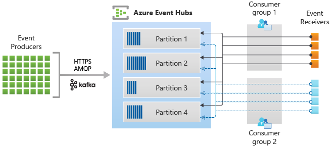

Leave a comment